
Up till now, I’ve been using power series to parametrize branches:
x(t) = a0+a1t+a2t2+ ⋯, y(t) = b0+b1t+b2t2+ ⋯
If the branch passes through the origin, then a0=b0=0. In the last post, we established Facts 4 and 5, assuming that y(t)=t for all branches, so x(t) = a0+a1y+a2y2+ ⋯.
That special assumption doesn’t always hold. As a fairly simple example, take this blue circle tangent to the x-axis:
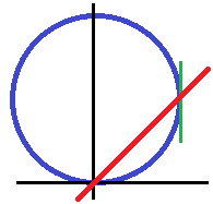
x2+(y–2)2=4
(Ignore the red and greeen lines for a moment.) Solving for x in terms of y, we get 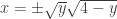


In this case, we could switch the roles of x and y, getting the two branches 

Even with a single curve, we could be in trouble. Consider the semicubical parabola y2=x3 (see Kendig Example 3.11, p.55):

y2=x3
We have either 
![x=\omega^i\sqrt[3]{y^2}](https://s0.wp.com/latex.php?latex=x%3D%5Comega%5Ei%5Csqrt%5B3%5D%7By%5E2%7D&bg=ffffff&fg=333333&s=0&c=20201002)
The solution: fractional power series, aka Puiseux series. For the circle, we have near 0

and for the semicubical parabola,


Perhaps you have qualms about the ambiguity of n-th roots (as I did at first). In the next post, I will try to dispel these three ways: via extension fields, via Riemann surfaces, and via the theory of fractional power series. We’ll see that the ambiguity plays an essential role.
First let’s see how Facts 4 and 5 work out with this technique. Along the way, we’ll see how it squashes the “grade inflation bug” mentioned way back in post 3.
You can paper over the fractional exponents using a so-called uniformizing parameter t. For the circle, use t=y½, giving 


If we stick with fractional exponents, the multiplicity calculation looks like this: the parametrization is

and F(x,y)=y. The equation F(x,y)=y=ϵ has only a single solution for any ϵ, but x≈2ϵ½ has two possible values because of the ambiguity of the square root, when ϵ≠0. So we get two intersections when we perturb things slightly.
As an instructive comparison, let F(x,y)=y–x be the red diagonal line. Plugging in the parametrization now gives F(x,y)≈y–2y½. Before we had two values of x for one value of F. Now we have two values of x for two values of F (near but not at O), because both have y½ as their lowest power of y. One F for one x, multiplicity 1.
Let’s generalize. If E(x,y) is monic as a polynomial in x, then any branch crossing the x-axis has a parametrization

with ak≠0 and all the exponents having the same denominator d (see Kendig §3.4, p.54). As usual, we care only about the lowest-order term, so assume that k and d are coprime—it doesn’t matter if higher-order exponents require a larger denominator. Clearly the lowest-order term of F(xE,yE) will have the form 
This is a good spot to discuss conjugate parametrizations (see Kendig p.55). The parameter t belongs to the family of d conjugate parameters t, ωt, …, ωd–1t, where ω is a primitive d-th root of unity. As t “fills out” a small disk |t|<δ in the complex plane, so do all of its conjugates (as Kendig puts it). Since y=td, all the conjugate values give the same y, but different x‘s. We get the same branch, in the sense of the totality of (x,y) values, but d different parametrizations of it.
It’s particularly easy to picture all this for the blue circle above, since d=2 and the conjugate values are ±t. Restricting attention to real values of t near 0, one parametrization traces a small arc of the circle near O from left to right, the other from right to left. For the level curves which are lines parallel to the x-axis, two values of t land on the curve; for the level curves which are lines parallel to the red line, only one (keeping t small).
We have to make almost no changes to this argument when k≠1, provided k is still coprime to d (as assumed). We still get d different values of x for the d values of t and that’s all we need. A little number theory furnishes the proof of this claim. Namely, the exponents of ω essentially belong to the ring ℤ/dℤ, and k is a unit in that ring: lk≡1 mod d for some l, since gcd(k,d)=1 implies lk+qd=1 for some l and q. That means that as j ranges from 0 to d-1, (ωjt)k=ωkjtk takes on d different values. Incidentally, the need for k to be coprime to d prevents the grade inflation bug: replacing d with a multiple is forbidden.
Very good, we now understand multiplicity when using fractional power series. How about the proof of Fact 4? Once again we consider the formula

where we assume that the leading coefficient am is a constant, and the x-degree of E is m, of F is n. Key point: the ui(y)’s must include all the conjugate parametrizations of each branch. Otherwise we won’t get m of them! (See Kendig pp.55–56. We saw a similar situation in post 10 with the two-ellipse example: we had to include both positive and negative square roots in the factorizations.)
Among the E-branches crossing the x-axis, we might find all sorts of denominators d. (When d=1, we have the special case treated in the last post.) We need to show that an E-branch intersecting F with multiplicity r on the x-axis, contributes a factor of yr to the lowest-order term in eq.(2). Multiplicity r means that the lowest-order term of F(ui) looks like cyr/d. With all its d conjugates, we get a contribution of (yr/d)d. All’s right with the world!
Finally, Fact 5 follows from Fact 4 just as in the last post.
