Algebraic Geometry Jottings 17

Prev TOC Next

At last we come to Kendig’s proof of Bézout’s Theorem. Although not long, it will take me a few posts to appreciate it in full.

Kendig starts by choosing favorable coordinates; among other desiderata, he wants to avoid intersections at infinity. From the standpoint of logical efficiency, this is the right call. But I’d rather go through these difficulties than around them, as much as possible, hoping to glean more insight.

Another complication: fractional power series (Puiseax series). Kendig introduces these in §3.3. I’ve been avoiding them, and I prefer to postpone the reckoning for one more post.

The argument, thus modified, has four steps.

1. Show Facts 4 and 5 from post 15: the order of the resultant is the sum of the multiplicities on the x-axis (with some provisos), and the degree of the resultant is the sum of all multiplicities in the affine plane (same provisos).
2. Adapt (1) to handle fractional power series.
3. Homogenize E and F and show how the homogenized resultant now counts the intersections at infinity as well.
4. Show that the homogenized resultant has degree mn.

As usual, I’ll chew over the details.

Recall Kendig’s first definition of multiplicity, for a branch of E at an intersection with the curve F at the origin O. (For another intersection point P, move P to O.) First assume we’ve parametrized the branch via power series in a variable t, (x_E(t),y_E(t)). Plug into the polynomial F(x,y) getting a power series F(t) = F(x_E(t),y_E(t)). The order of F(t)—the degree of its lowest order term—is the multiplicity of the branch-curve intersection. Post 3 explored the intuition behind this: when we “perturb” E or F or both a little, an intersection of multiplicity r typically splits into r distinct intersections.

Remember also the local-global feature of Bézout’s Theorem: we need to total up all the branch-branch multiplicities at an intersection, and then sum this over all intersections. Kendig’s first definition already sums over the branches of the curve F. The second definition sums over horizontal lines when using res_x(y), or vertical lines when using res_y(x). For example, the roses:

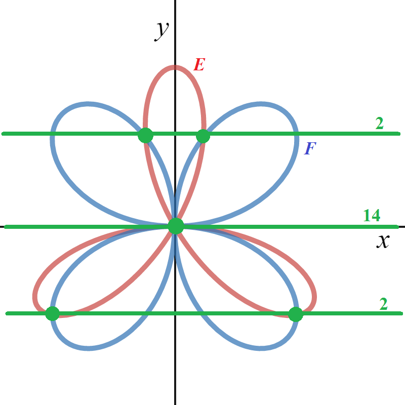
res_x(y)=16y¹⁴(16y²-5)²

The green horizontal lines pass through the intersections; the green numbers at right are total multiplicities. As we’ve seen before, res_x(y)=16y¹⁴(16y²-5)² has order 14, for the single intersection of multiplicity 14 on the x-axis. The top horizontal line has y-coordinate √5/4; we shift it down to be the new x-axis by substituting (y+√5/4) for y in the resultant. It would be painful to expand the result by hand, but we care only about are the lowest degree terms of 16(y+√5/4)¹⁴, clearly a nonzero constant, and (16(y+√5/4)²-5)², easily computed to be a constant times y². So we get total multiplicity 2 for this line. Likewise for the bottom horizontal line.

Recall the formulas for the resultant:

    (1)
    (2)

E(x,y) = a_m(y)x^m+···+a₀(y) = a_m(y)(x–u₁)···(x–u_m)    (3a)
F(x,y) = b_n(y)xⁿ+···+b₀(y) = b_n(y)(x–v₁)···(x–v_n)        (3b)

(I’ve made it explicit that the coefficients are polynomials in y.) Kendig proves Fact 4 (or rather a special case) using (1), but I prefer to use (2). The branches of E crossing the x-axis are essentially just the roots of the equation E(x,y) = 0; let’s assume these can be expressed as power series in y for y small enough. (This won’t work if a branch isn’t locally the graph of a function, but I’m postponing that issue.) Thus the i-th branch has the parametrization (u_i(y),y), where u_i(y) is a power series in y. In other words, we have a parametrization (x,y) = (u_i(t), t).

By Kendig’s first definition, the multiplicity of the intersection between the i-th branch of E and the curve F is just the order of F(t) = F(u_i(t), t) in t. Since y=t, this is just the order of F(u_i(y), y) as a power series in y. When you multiply power series, the orders add. Therefore, by eq.(2), the order of res_x(y) in y is the sum of the multiplicities over all branches of E crossing the x-axis, plus n times the order of a_m(y). If a_m(y) is a constant, we get Fact 4 as stated.

How about the other horizontal lines? To get their y-coordinates, we factor the resultant, say

res_x(y) = k(y–c₁)^r₁···(y–c_l)^r_l

If, say, c₁=0, then r₁ would be the order of res_x(y), measuring the contribution from the x-axis. If c₁≠0, then we shift things up or down to make it the x-axis, by substituting y+c₁ for y. This works for any c_i. We conclude that r_i is the total multiplicity of the intersections on the line y=c_i (when a_m(y) is constant). Since r₁+···+r_l is the degree of res_x(y), we’re done!

Prev TOC Next