The Speed Law
Kepler initially believed in the inverse distance speed law. I’ve discussed how he argued that his whirlpool force hypothesis provided the physical explanation for Ptolemy’s equant. Now we’ll look at the transition to the area law.
First though a change in perspective. Kepler did not have the calculus concept of instantaneous velocity. Informally he did use terms like “swiftness” (celeritas). But for computations, he worked either with the delay: the time to traverse a given small length of the orbit. Or else, inversely, the length traversed during a given small time interval. Initially he used the delay. For this reason, several authors refer just to the “distance law” instead of the “inverse distance speed law”. I’ll do the same in this post.
Delay makes sense when we reflect on the astronomer’s goal: to predict when the planet will appear at a given position. The computational procedure: starting with the planet at aphelion, divide the orbit into many small segments; then add the delays for each segment, each delay proportional to the distance. Determine the constant of proportionality by doing this for the entire orbit, and comparing the result with the known period.
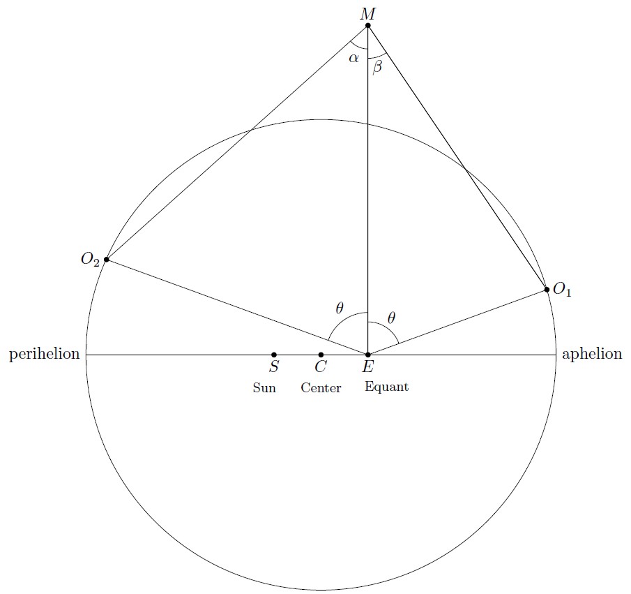
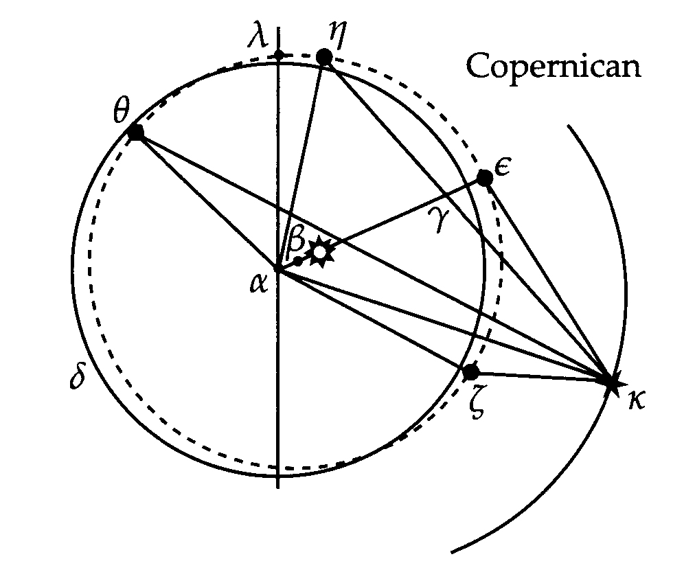
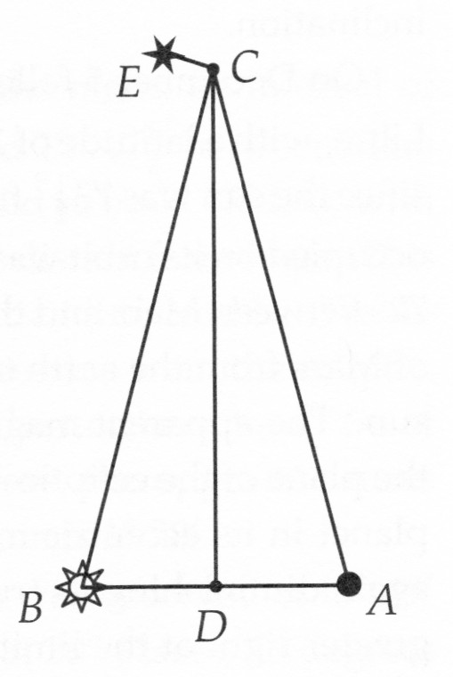
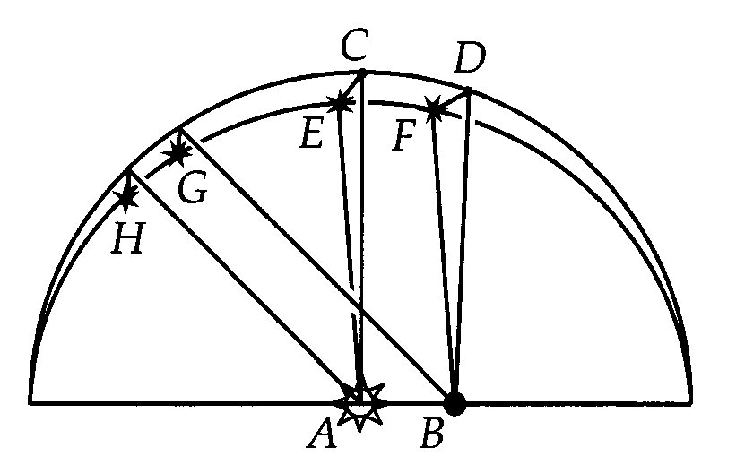
Kepler does this in Chapter 40, chopping the orbit of Mars (still assumed circular) into 360 parts, each subtending a central angle β of 1°. (See the left side of the figure below.)

Sum of the Radii, and the Area Law
Say ri is the Sun-Mars distance at i degrees from aphelion. So Kepler is calculating the time for Mars’s arrival at that position with this formula:
tn=∑i=0n ri Δβ / ∑i=0360 ri Δβ
Δβ is proportional to the length of the segment Δs, because β is a central angle. So each term is proportional to the delay.
You may recognize these sums as Riemann sums for integrals ∫r dβ. Of course Kepler did not have integral calculus to draw on, but he did have Archimedes. He wrote:
… since this procedure is mechanical and tedious … I looked around for other means. And since I knew that the points of the eccentric [i.e., the orbit of Mars] are infinite, and their distances are infinite, it struck me that all these distances are contained in the plane of the eccentric. For I had remembered that Archimedes, in seeking the ratio of the circumference to the diameter, once thus divided the circle into an infinity of triangles … Accordingly, instead of dividing the circumference, as before, I now cut the plane of the eccentric into 360 parts by lines drawn from the point where the eccentricity is reckoned [C in my diagram].
A word about what I will call the sunny side of presentism. Kepler did not have calculus in his toolbox, or even algebra, but dealt with geometrical close equivalents. It illuminates matters to place the modern1 approach alongside his.
So, he is trying to find t as a function of s, the length traveled. His distance law becomes dt/ds∝r instead of ds/dt∝1/r. Thus t∝∫r ds. The area of a central sector (like ACM) is proportional to the length of the arc (AM here). Each of these central “triangles” has base ds=Rdβ and altitude R, thus area proportional to R2dβ.
Kepler now extends this to sectors from the sun, like ASM. The area of ASM, he argues, should furnish a measure of the sum of the Sun-Mars radii—that is, of the delay along the arc.
This area is easily computed: just divide ASM into the central sector ACM and the triangle △CSM. The eccentricity CS is eR, and △CSM has base eR and altitude R sinβ. If β is measured in radians, then the area is 1/2 R2(β+e sinβ).
Let’s see how integral calculus views this. The “infinite sum of radii” is ∫r dβ, or maybe ∫r dθ. (When the eccentricity is small, dβ≈dθ, so it shouldn’t matter much.) An infinitesimal element of area is 1/2 r2 dθ (see the right side of the figure above). For small eccentricity r≈R, so
1/2 ∫r2 dθ ≈ 1/2 R∫r dθ
Therefore the sum of the radii is proportional to the area, approximately.
Kepler recognized that his equivalence was not exact:
Nevertheless, my argument contains a paralogism, not, indeed, of great moment. It arises from this: that while Archimedes did indeed divide the circle into an infinity of triangles, they stood upon the circumference at right angles, so that their vertices were at the center of the circle C. But one cannot proceed in the same way with triangles standing upon the circumference with their vertices at S, because the circumference is intersected obliquely by the straight lines from S in all places other than aphelion and perihelion.
[I have edited this slightly to match my diagram.]
He discovered the inexactness from a brute-force calculation. He also provided a demonstration that the sum of the radii over the whole circle is greater than the area. See the figure below:
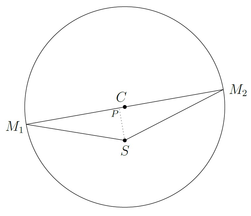
Sum of Radii greater than the Area
Pair the radii as indicated, SM1 with SM2 and CM1 with CM2. Here M1 and M2 are the two ends of a diameter. The triangle inequality tells us that SM1+SM2 is greater than the diameter M1M2. But the sum of the diameters should give us the area of the circle.
Note that if you drop a perpendicular from S to the diameter (the dotted line SP), then the sum PM1+PM2 will equal the diameter. Kepler called PM1 and PM2 the diametral distances. They were to play an crucial role in the discovery of the elliptical orbit.
A page or so after the passage quoted above, Kepler says:
[this method] agrees most precisely with the observations in the theory of the sun or earth. Nevertheless, it errs in two respects. First, it supposes that the orbit of the planet is a perfect circle, which, as will be demonstrated below in Ch.44, is not true. Second, it uses a plane [i.e., area] which does not exactly measure the distance of all points from the sun. Nevertheless, as if by a miracle, each of these exactly cancels the effect of the other, as is demonstrated below in Ch.59.
Translator Donahue notes: “Readers who hope to find a clear explanation in Ch.59 will be disappointed”, and he describes the treatment there as “no more than qualitative gropings towards a solution”.
The transition from the distance law to the area law
The transition involved several points.
(1) Suppose instead of having dt∝r, we let dt be proportional to the diametral distance. This is R+eR cosβ (see figure below):
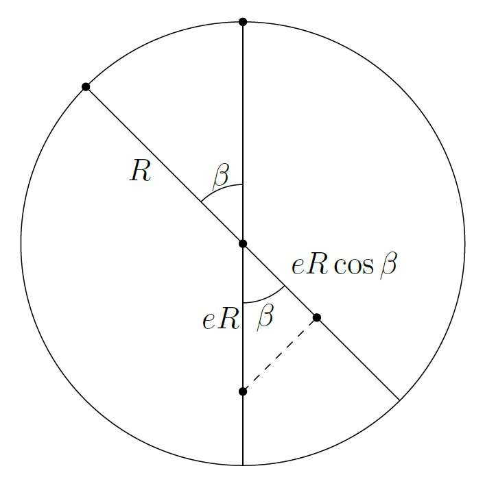
Diametral Distance
So t is proportional to ∫(1+e cosβ)dβ=β+e sinβ. As noted above, the area is 1/2 R2(β+e sinβ). Thus t is proportional to area, if we replace the radial distance from the sun with the diametral distance.
(2) Kepler understood this geometrically. The correct formula for the area of each small triangle in our first figure (with vertex at the sun) is 1/2 base×altitude, not 1/2 base×side. But the altitude of the small triangle is the diametral distance. So the area precisely measures the “infinite sum of diametral distances”.
(3) Spoiler alert! Kepler ultimately concluded that the Mars-Sun distances are the diametral distances. Hence the area precisely measures the “infinite sum of distances to the ellipse”.
(4) Now we have an odd situation. We have the eccentric circle. The actual orbit is an ellipse inside it, tangent to the circle at the apsides. But the slogan “equal areas in equal times” refers to the areas of sectors of the circle, not the ellipse.
This is easily fixed. The ellipse is a “squished circle”, obtained from the enclosing circle by the transformation (x,y)↦((b/a)x,y). (Here b and a are the semi-minor and semi-major axes.) That means that proportional areas remain proportional, the times are still proportional to the elliptical areas swept out, and the slogan still works.
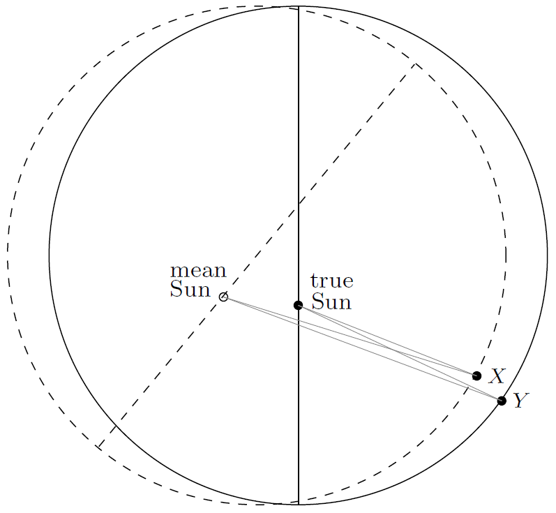
(5) We still have one problem. Kepler drew radius vectors from the sun to the orbit, and spaced them using the central angle. In other words, the areas are proportional to ∫r dβ, where r now is the Sun-Mars distance with Mars on the ellipse. But this disagrees with the distance law. That says dt/ds∝r, so t∝∫r ds. For the circle, ds=Rdβ, so the proportionalities hold using either dβ or ds. Not true for the ellipse: ds≠r dβ because the radius vectors are no longer perpendicular to the curve.
In Keplerian geometrical terms, his distance law says: for equal length segments, the delay is proportional to the radial distance. Yet here he is dividing the ellipse into unequal segments. Not kosher!
But if we resolve ds into radial and transverse components—say dsr and dsθ—then dsθ=r dβ. In fact r2 dβ is twice the area element, so ∫r dsθ=∫r2 dβ is both the measure of the delay and twice the area of the sector.
Looked at another way, it is just the transverse speed, vθ=dsθ/dt, that is inversely proportional to the radial distance.
This makes sense physically. The “solar whirlpool” has no radial component of force. It acts purely transversely on the planet. Go way back to the evidence that suggested it: the speeds at the apsides are inversely proportional to the distances. But at the apsides there is no radial component.
Upshot: the physics agrees with the geometrical analysis. The area law reigns supreme.
From the Astronomia Nova to the Epitome
Ch.59 contains “Protheorems” to justify the elliptical orbit and the distance law. These demonstrate points (1)–(4) above.
I quoted Kepler earlier saying that his two errors canceled exactly. By this he means point (3), not a literal cancellation of quantities.
Ch.59 also shows that Kepler recognized the lack of equivalence between the distance law and the area law. He expresses it as I did above, that equal segments on the enclosing circle do not correspond to equal segments on the ellipse. He then gives a confusing argument why one should use the former. Accepting this change makes the distance law equivalent to the area law, as we’ve observed.
I think this counts as more than “qualitative gropings towards a solution”; Donahue undersells Kepler’s achievement. However, it still falls short of his final explanation, in the Epitome.
In that treatise, Kepler identifies two forces at work:
For it has been said above that, if the orbit of the planet is divided into the smallest equal parts, the times of the planet in them increase in the ratio of the distances between them and the sun. But this is to be understood not of all equal parts as such, but principally of [the apsides]….But in the case of the other parts which face the sun obliquely, this is to be understood only of that which in any of these parts belongs to the movement around the sun. For since the orbit of the planet is eccentric, therefore in order to form it two elements of movement are mingled together, as has been demonstrated already: one element comes from the revolution around the sun by reason of one solar virtue; the other comes from the libration towards the sun by reason of another solar virtue distinct from the first. [Translation by Aiton (p.88)]
Kepler’s “movement around the sun” refers to dsθ, so Kepler is saying that for equal dsθ’s, the dt’s are proportional to the distances. In other words, dt/dsθ is proportional to r, or dsθ/dt=vθ is proportional to 1/r.
Let’s write Fθ for the whirlpool force and Fr for the libration force. As I said above, it makes sense that Fθ would be proportional to vθ and not to v. The proportionality Fθ∝1/r formed a cornerstone of Kepler’s physics. Kepler regarded the change from ds to dsθ as correcting an oversight, preserving the essential features of his system.
In the Epitome Kepler also returns to the matter of inverse square vs. inverse linear. The Epitome is written in a Q&A format. Here’s the quote:
But if the light is attenuated in the ratio of the squares of the intervals, i.e., in the ratio of the surfaces; why therefore does not the motor virtue too become weaker in the ratio of the squares rather than in the simple [ratio]?
Because the motor virtue has as subject a form from the solar body, not according as it is merely body but according as it is set in motion in a revolution around its immobile axis and poles.
Therefore even if the form from the solar body is attenuated in longitude and in latitude no less than the light is; nevertheless this attenuation contributes towards the weakening of the motor virtue only by reason of the longitude: for the local movement which the sun gives to the planets takes place only in longitude, wherein even the parts of the solar body are mobile, not also in latitude towards the poles of the body with respect to which the sun is immobile. [Translated by C.G. Wallis, who uses “form” to translate the Latin species, rendered “image” by Stephenson and left untranslated by Donahue.]
We saw in post 21 the key to the matter: the whirlpool force has only cylindrical symmetry, not spherical. Kepler shows awareness of the issue and its resolution. Stephenson puts it this way:
As we have seen in the Astronomia nova, Kepler believed this force to vary inversely with distance from the sun. He carefully justified this relation in the Epitome, arguing that it was in fact reasonable for the motive force to follow a different law than light. He based his argument upon a distinction between “the immaterial image of the solar body, flowing out to the planets and beyond”, and “its force or energy, which close at hand grasps and moves the planet”. The image, although immaterial, was the subject for the force. As it spread through all the universe, the image suffered attenuation just as did light, in the squared proportion of distance from the source. In contrast, the force was not a substance (not even an immaterial substance), but merely an attribute, a virtue or ability, which the solar image possessed when in contact with the body of a planet. In empty space, where the image was spreading out and thinning as it expanded, there was no motive virtue, and hence no question of its weakening. The virtue came into play only where the sun’s image moved through a planetary body. It acted in one direction only, the direction of the sun’s rotation around the zodiac, and it was weakened only insofar as its subject, the moving solar image, was thinned out in this one direction. The motive effect of the sun’s image, therefore, decreased in simple inverse proportion to distance from the sun. [Stephenson (pp.142–143)]
Before leaving the topic of the speed law and the whirlpool force, let’s cite again their relation to Newtonian physics. In their final form, Kepler’s assumptions read: Fθ∝1/r and Fθ∝vθ. So vθ∝1/r, that is, vθr is constant. Angular momentum is mvθr, which Newtonian physics tells us is conserved. Mathematical equivalence!
[1] Modern!? Only 300 years old instead of 400!

 ;
; ;
;