Prev TOC Next
The Vicarious Hypothesis
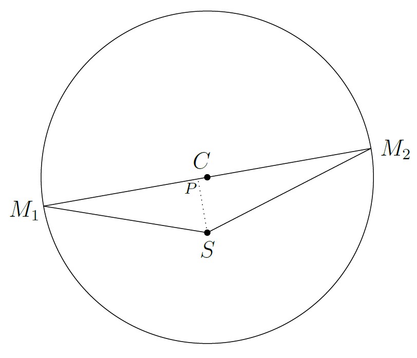
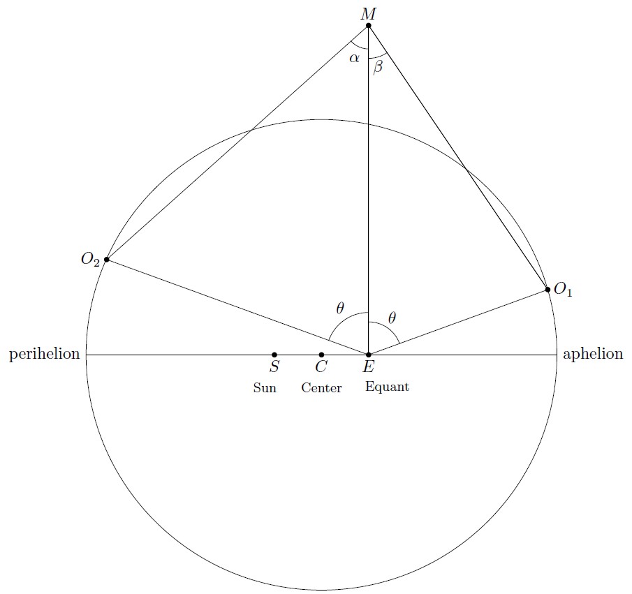
Part II of the Astronomia nova bears the title “Imitation of the Ancients”. Kepler obtains a model for Mars with an eccentric circle and an equant. But the eccentricity is not bisected. Instead, the center is closer to the equant than to the sun. See the figure below. (Notation: S=Sun, C=Center, E=Equant, r=radius, eS=SC/r, and eE=EC/r.)

The Vicarious Model
As this post is a bit long, let me highlight the main points.
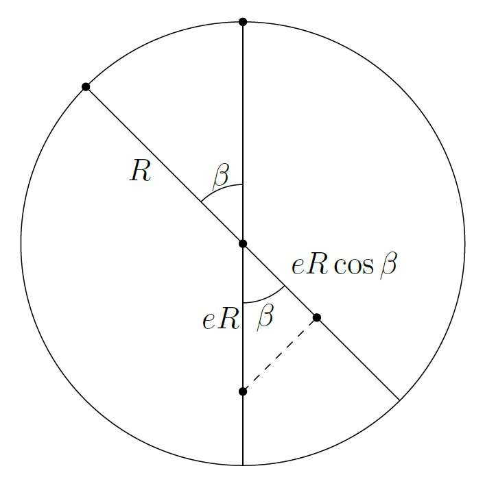
- The general model has parameters eS and eE. We always have eS+eE=2e, where e is the eccentricity.
- We get the best fit for heliocentric longitudes using the ratio eS:eE=5:3. This is quite close to Kepler’s vicarious hypothesis.
- We get the best fit for latitudes and “off to the side” observations with eS=eE, the famous “bisection of eccentricity”. It’s longitudes or latitudes, you can’t have both! At least with a circular orbit.
- Kepler determined the parameters for his vicarious hypothesis by an intricate double iteration, using four acronychal observations.
- The whirlpool force hypothesis requires bisection of eccentricity.
- Although Kepler ultimately rejected the vicarious hypothesis as the correct model, he continued to use it to compute heliocentric longitudes. This is an implicit appeal to his “zeroth law”.
A Modern Perspective
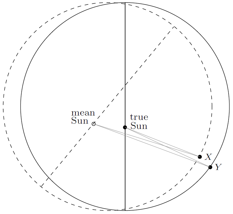
I will refer to the scheme of the figure above as the vicarious model; Kepler used this term for a particular choice of parameters. By the “elliptical model”, I mean the usual elliptical orbit with the planet obeying the area speed law. I assume throughout that the period is the same for both models.
Before considering what Kepler wrote and did, we’ll examine the two models with modern techniques.
Suppose all we care about are heliocentric longitudes. We want to choose the parameters in the vicarious model to match these as accurately as possible. We don’t care about latitudes or distances. Observationally, this means we look only at acronychal measurements of the geocentric longitude. For as noted in post 24, when the planet is in opposition, the heliocentric and geocentric longitudes are equal.
What parameters will make the vicarious model best approximate the elliptical model for heliocentric longitudes? Evans and Linton (p.179) derive the answer: eS+eE=2e where e is the eccentricity of the ellipse, and eS:eE=5:3.
Evans obtains this result several ways. He imposes three conditions on the motion. Let P be perihelion, and Q quadrature (i.e., the point such that PSQ is a right angle). First condition: the time from perihelion P to Q must be the same for both models. To an excellent approximation when e is small, this implies that eS+eE=2e.
Second condition: the angular speed at aphelion must be the same for both models. This gives the equation
 ;
;
retaining only terms up to order e2, this becomes
eS+eE = 2e+2eeS−5/2e2
Third condition: the angular speed at perihelion must be the same for both models. By similar reasoning, we have
 ;
;
approximated to
eS+eE = 2e−2eeS+5/2e2
So we have three equations: eS+eE=2e, and the aphelion and perihelion angular speed results. Any two of these equations yields eS:eE=5:3.
Evens gives another derivation, using an expression for the heliocentric longitude measured from perihelion as a function of time. (Linton gives essentially the same derivation, but using aphelion instead of perihelion.) Let this be θ, and let ω be the average angular speed, i.e., 2π/T. Up to second order in e, the expression is
θ(t) = ωt+2e sin ωt+5/4e2 sin 2ωt
for the elliptical model, and
θ(t) = ωt+(eS+eE) sin ωt+½eS(eS+eE) sin 2ωt
for the vicarious model. So first: when eS+eE=2e, the expressions agree to first order in e. Second: when also eS:eE=5:3, we have eS=5/4e, and so they agree to second order.
In short, the vicarious model gives very good heliocentric longitudes when eS:eE=5:3. To quote Evans: “In fact, with the precision achievable with naked-eye observations even in Kepler’s day, there is no perceptible error in the angular position anywhere around the orbit—as Kepler himself verified.”
Okay, what if we do care about distances and latitudes? Geocentric latitudes provide a means to determine distances. I’ll explain this in more detail below, but intuitively: the closer you are to Mars, the bigger the latitude looks. An optical effect, just like approaching a vertical pole and seeing it look taller. Viewing Mars out of opposition, “from the side”, furnishes another way to check actual distances.
Perihelion and aphelion are minimal and maximal Sun-Mars distances, so a vicarious model that tries to do a good job with distances will share the apsidal line with the elliptical model. That means they will also have the same center and same r, where r is the vicarious radius and the elliptical semi-major axis. In the elliptical model, the Sun-Mars distance at aphelion is r+e and at perihelion is r−e. In the vicarious model, these distances are respectively r+eS and r−eS. Conclusion: the vicarious model gives the correct Sun-Mars distance at aphelion and/or perihelion only when eS=e. In other words, the eccentricity must be bisected.
The upshot: using the scheme of the above figure, you are faced with Scylla and Charybdis. You can have an excellent model for finding heliocentric longitudes at any time, all around the orbit. Just choose eS:eE=5:3. Or you can have a model for distances that is accurate at aphelion and perihelion. Choose eS=eE=e. You can’t have both.
One more observation: if we do bisect the eccentricity, then the two expressions for θ(t) will first disagree at order e2. That is, in the term with the factor sin 2ωt. The maximum (absolute) value occurs when 2ωt=±π/2. Since 2ω=4π/T, that means at t=±T/8. For small eccentricity, this is close to the octants.
What Kepler Did
After some preliminaries, Kepler gets down to business in Chapter 16 of the Astronomia nova. It takes four parameters to specify a vicarious model: the two eccentricities eS and eE, the direction of aphelion, and a time when the planet is at aphelion (known as the epoch). Kepler used four acronychal observations to derive the parameters.

Determining the Vicarious Parameters
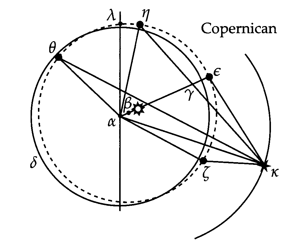
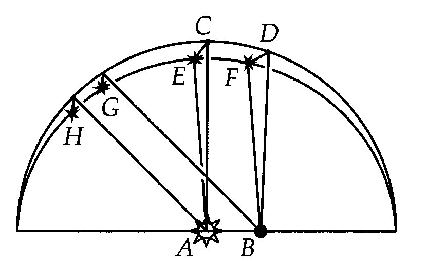
The left of the figure above is Kepler’s diagram; the right side removes some clutter. A is the sun, B is the center of the orbit, and C is equant. D, E, F, and G are the four acronychal observations. They give us heliocentric longitudes: the directions of the lines AD, AE, AF, and AG. The directions from the equant (CD, CE, CF, and CG) are called mean longitudes. Since we know the times of the observations, we would know the mean longitudes if we knew the epoch and the direction of aphelion. That’s because the planet moves uniformly when viewed from the equant, and we know the period. Referring to the right side of the figure, you can see that we’d have two angles of the triangle AGC; of course, this also holds for the other three triangles. Temporarily chose the distance unit so that AC has length 1. Then we can solve all these triangles and find the positions D, E, F, and G.
Kepler imposed two constraints. First, the four acronychals must lie on a circle. This is easily checked, since a quadrilateral is cyclic if and only if opposite angles add to 180°. Also, the center B of the circle must lie on the line segment AC. If these are met, then we can determine both the radius and the center of the circle. That gives us the two parameters of the vicarious model, AB/r=eS and CB/r=eE.
Unfortunately, there is no direct way to find the epoch and direction of aphelion from the acronychals. Kepler proceeded iteratively. Starting with an estimate for these two quantities, he computed the positions DEFG. If these failed the circle requirement, he adjusted the direction of aphelion. “Repeat until done”, i.e., until DEFG lie on a circle. Gingerich (Ch.22) calls this the “inner iteration”. Then Kepler checked that B lay on the line segment from A to C. If not, he adjusted the epoch. This is the “outer iteration”, since the aphelion direction must now be recomputed. Eventually the process converged on values with both requirements satisfied. Kepler’s final result: eS:eE=18564:11332≈4.91:3.
Gingerich (Ch.22) and Voelkel (pp.106–107,111,114–121) present the whole messy story, based on Kepler’s copious manuscripts. In contrast to the account in the Astronomia nova, Kepler began in 1600 by tackling the earth’s orbit (i.e., revising Tycho’s solar theory). In the same year he made his first assault on the orbit of Mars. The two investigations continued in a tangled fashion, with interruptions, until sometime in 1602.
Downfall: Down but not Out
In Chapter 18, Kepler proclaims victory:
You see then, O studious reader, that the hypothesis found by the method developed above, is able in its calculations to account, in turn, for the four observations upon which it was founded, but also to comprehend all the other observations within two minutes…
And Chapter 19 begins:
Who would have thought it possible? This hypothesis so closely in agreement with the acronychal observations, is nonetheless false…
Chapters 19 and 20 then show, “with great thoroughness and almost masochistic delight” (Koestler (p.322)) that the vicarious hypothesis disagrees with geocentric latitudes and observations out of opposition.

Geocentric Latitude
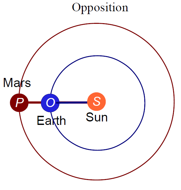
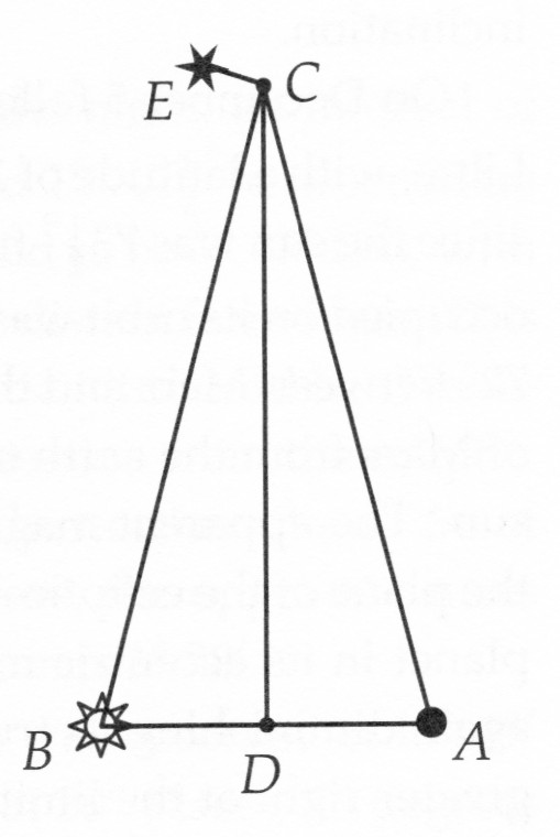
We’ve already seen all the ingredients. First, latitudes. Consider the Sun-Earth-Mars triangle (see figure above). At opposition this lies in a plane perpendicular to the earth’s orbit (the ecliptic). The inclination of Mars’s orbital plane is the angle Earth-Sun-Mars. The geocentric latitude is the supplement of the angle Sun-Earth-Mars. If you know the Earth-Sun distance, then you can solve the triangle and get the Sun-Mars distance.
Kepler does this in Chapter 19, and concludes that the Martian eccentricity is between 0.08000 and 0.09943; his vicarious hypothesis sets it at 0.11332. He also notes that “combined eccentricity” (i.e., from the sun to the equant) is about 0.18564; half that is 0.9282, or just about the mean between 0.08000 and 0.09943.
Chapter 20 looks at some longitudes when Mars at perihelion and aphelion, but Earth is “off to the side”—that is, away from opposition. Again the results refute the vicarious model, and fit a bisected eccentricity rather well.
Puzzling. Kepler anticipates the resolution: “the orbit of the star is not a perfect circle, but an oval…”
Although the vicarious hypothesis failed, it still provides Martian longitudes to an accuracy of 2′. Kepler uses it for this purpose in subsequent chapters. In other words, Kepler assumes that if the earth were in opposition, instead of off to the side, then the vicarious longitudes would be correct.
Note the implicit appeal to the zeroth law: No special treatment for the earth. The solar longitude of Mars can’t depend on Earth’s position. Okay, but why prefer the acronychal (opposition) data to the off-to-the-side data?
Answer: the longitudes in question are the Sun-Mars directions. An acronychal observation directly measures this, since the Earth-Mars and Sun-Mars directions are identical. This doesn’t hold for an off-to-the-side measurement. So we should trust the acronychal values, and the vicarious hypothesis gives those values with good accuracy around the whole of Mars’s orbit.
Feetnote
(1) The Mars model by Longomontanus, mentioned in post 24, used a Copernican epicyclet instead an equant (see post 20). But we can convert it into a nearly equivalent equant model; Evans shows how to translate the parameters. Under this transformation, the Longomontanus model had eS:eE=5:3.
(2) Kepler complains in Chapter 16:
If this wearisome method has filled you with loathing, it should more properly fill you with compassion for me, as I have gone through it at least seventy times at the expense of a great deal of time, and you will cease to wonder that the fifth year has now gone by since I took up Mars, although the year 1603 was nearly all given over to optical investigations.
Gingerich (Ch.21) wondered why it took Kepler 70 iterations. He programmed it, and it took the computer only 9 trials! He guessed initially (and wrongly) that “Kepler was horribly plagued by numerical errors”. But when he gained access to Kepler’s manuscripts (Ch.22), he found two causes: bad data, and Kepler’s treatment of redundant observations. Gingerich writes:
Thus we see that in the vicarious orbit solution Kepler worked always with the same four oppositions, but the results were repeatedly tested against additional oppositions. In the course of five years’ work, the reduction of the basic data was continually improved. His 70 iterations were spent (probably) in five separate solutions differing only in the values chosen for the initial times and angles.
Gingerich also notes a fine point I glossed over in my account:
Tycho Brahe had no operational way of knowing precisely when Mars was at opposition. Tycho’s raw observations only approximated the opposition places, and Kepler was obliged to correct and interpolate them to obtain the acronychal positions he required.
(3) The whirlpool force explanation for the equant requires bisecting the eccentricity (see post 4 and post 20). So in considering the vicarious model at all, Kepler tempered his commitment to this hypothesis.
Voelkel (pp.107–111) found confirmation in a document Kepler wrote around 1602. We’ve noted how the inverse distance speed law works tolerably well within an orbit, but fails when comparing different orbits (see post 20). In the document, Kepler notices his earlier errors in this matter.Voelkel suggests that this realization freed Kepler to study other divisions of eccentricity. It must have come as a relief when the latitude and off-side computations indicated that eccentricity should be bisected.
Prev TOC Next