Category Archives: Math

Set Theory Jottings 25. Mostowski Collapsing Lemma

Prev TOC Next

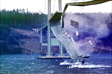
The Collapse of the Tacoma Bridge

A relational system is a pair (A,R) where A is a class and R is a relation on A. If R has certain properties, we get a mapping (the Mostowski collapsing map) F:AM from A to a transitive class M. F is an isomorphism, in this sense: yRx if and only if F(y)∈F(x). If yRx, we say y is a component of x, and we write x* for the class of components of x.

Here are the properties we demand of (A,R):

  • Extensionality: For all x,y in A, if xy then x*≠y*.
  • Properness: For all x in A, x* is a set.
  • Well-foundedness: R is well-founded, i.e., every subclass of A has an R-minimal element.

If we drop extensionality, we can still define the Mostowski map F, but we no longer get an isomorphism.

An important special case: R is ∈. In this situation, x* is the set of elements of x that belong to A; in other words, Ax.

It helps to think of the elements of A as names or labels for sets. The Mostowski mapping xF(x) sends the name x to the named set F(x). The following fact defines F, as we will see:

F(x)={F(y):yRx}  (Eq.1)

That is, you recursively apply F to each component of x, and gather the results into a set. So:

The names of the elements of F(x) are the components of x.

Note that if an element x has no components, then Eq.1 says that F(x)=∅.

Let’s look at an example, then see how to justify these claims.

Figure 1: A Mostowski Map

Fig.1 illustrates the Mostowski mapping F for a relational system (A,R). All the R-edges are explicit: although bRdRe, we do not have bRe.

Here a is a name for the empty set, since it has no components. The only component of b is a, so b*={a} and F(b)={F(a)}={∅}=1. Likewise for the rest of the figure. Here is all of F:

a↦∅
b↦{∅}=1
c↦{∅,1}=2
d↦{1}
e↦{{1}}
f↦{{1},2}

Another example, based on Fig.1: let R=∈. Let a be some random set, say ω. That makes ω a name for the empty set in this system. Also b={ω}, while F(b) is still {∅}. Likewise for the rest of the figure. (Exercise: what is f? What is F(f)?)

If we add a couple of nodes (a′ and c′) to Fig.1, we get the non-extensional system of Fig.2 below. Note that a′ has the same components as a. This single failure of extensionality propagates upwards: while c and c′ have different components, they still map to the same set because a′ and a both name the same set. The Mostowski map is no longer an isomorphism.

Figure 2: A Non-extensional Mostowski Map

The map is the same as in Fig.1, plus a′↦∅ and c′↦{∅,1}=2.

Next, let’s see why Eq.1 defines a function on all of A. I don’t want to get bogged down in details, so I’ll just sketch the reasoning. We define the descendants of xA just like the transitive closure in post 14: let s(x)=x*, and then desc(x) = x s(x) ∪ s2(x) ∪···∪ sn(x) ∪ ···.

Say that uA is good if there is a function fu with domain {u}∪desc(u) satisfying Eq.1:

fu(x)={fu(y):yRx} for all x∈{u}∪desc(u)

If uA is not good, we say it is bad. By the well-foundedness of R, if there are any bad elements in A, there is an R-minimal one, say u. So all the components of this bad u are good. Next we show that if v1 and v2 are components of x and fv1 and fv2 are the functions satisfying Eq.1 on their respective domains, then the functions agree on the overlap—on the intersection of the domains. If not, there is an R-minimal element (say t) where they disagree. But then Eq.1 shows that they have to agree on t as well.

This means that we can “meld” all the component fv’s together, to get a function defined on all descendents of u. But then we can use Eq.1 to define the function on u as well, satisfying the equation throughout, and u wasn’t bad after all.

Finally we define F with domain A by melding all the fu’s together.

Eq.1 obviously implies

yRxF(y)∈F(x)

Extensionality (not used till now) makes this an “if and only if”, and also implies that F is injective. Here’s why. Say x1x2 but F(x1)=F(x2). Since x1x2, one of the x’s has a component the other lacks; say y1Rx1 and ¬(y1Rx2). So F(y1)∈F(x1)=F(x2). But can we have F(y1)∈F(x2)? Only if there is a y2Rx2 such that F(y1)=F(y2). From x1x2 with F(x1)=F(x2), we’ve obtained y1Rx1, y2Rx2, with y1y2 and F(y1)=F(y2). An R-minimality argument shows this can’t happen, and so F is injective. Now suppose we have elements x and y with F(y)∈F(x). Eq.1 says that F(y) is F(y′) for some yRx. But injectivity tells us that y=y′, so yRx, as required.

Up top we mentioned the key fact about the Mostowski map:

The Mostowski map F is an isomorphism from (A,R) to (M,∈), where M is a transitive class.

Naturally we define M as the image of A under F, making F surjective, and so we have our isomorphism. What about transitivity of M? This is immediate: given any F(x)∈M, its elements are, by definition of F, of the form F(y). So they also belong to M.

We next look at the special case where R is ∈. As noted above, in this case x*=Ax. So (A,∈) is automatically proper because x* is contained in the set x. Well-foundedness also comes for free because of Foundation.

We focus on the interplay between extensionality and transitivity. Transitivity implies extensionality: if A is transitive, then x*=Ax=x, since x is an element of A and hence a subset of A. This shows even more: if A is transitive then F is the identity map. Proof: F(x)={F(y):yx*}={F(y):yx}, so by R-minimality of ∈ (or ∈-induction, see post 14), F(x)=x for all xA.

We can squeeze a little more juice out of this. Assume that B is a transitive subclass of A, with A perhaps not transitive. For any xB, x*=x because xBA. So the same argument shows that F is the identity on B.

Extensionality does not imply transitivity. When R is ∈, then all components are elements, but not all elements need be components.

For example, here’s a system (A′,∈) with the same graph as in Fig.1:

a={5}, b={a,6}, c={a,b,5}, d={b,7},  e={d},  f={c,5,7}

I started with the image of F (i.e., F(a)=∅, F(b)=1, etc.) as the “main ingredients”. I never said what a,b,c etc. were in Fig.1, so I let them be their images under F. Then I added 5, 6, and 7 as “spices” to some elements of A, without adding them as elements in their own right. The result is A′. Since the spices do not belong to A′, their addition doesn’t change the graph. So b’s only component is still a, c’s only components are still a and b, etc. The Mostowski map for (A′,∈) (call it F′) “de-spices” the dish. Result: F′(A′)=A. We have an extensional non-transitive system mapped to a transitive one.

At the end of post 24 I mentioned a reflection principle, which I now rephrase:

If K is a countable set and Φ is a finite set of ZF closed formulas (allowing parameters from K), then there is a countable set MK reflecting all the formulas in Φ.

Suppose that K contains a transitive subset K0. Add to Φ the Extensionality Axiom, “∀x,y(xy→∃z(zxzy zyzx))”. Apply the reflection principle to get an extensional relational system (M,∈) reflecting all of Φ. Apply the Mostowski map F to (M,∈) to get a transitive relational system (N,∈), ∈-isomorphic to (M,∈). The ∈-isomorphism implies that N also reflects Φ. F restricted to K0 is the identity by what we’ve said above. So K0 is a subset of N (although K might not be). Obviously N is countable. We conclude:

If K is a countable set containing a transitive subset K0, and Φ is a finite set of closed formulas in ℒK(ZF) (so allowing parameters from K), then there is a countable transitive set NK0 reflecting all the formulas in Φ. In reflecting the formulas of Φ, the parameters from K are replaced with images under an ∈-isomorphism; this ∈-isomorphism is the identity on K0.

This may seem rather complicated, but we will need it in a later post.

Prev TOC Next

Leave a comment

Filed under Set Theory

Set Theory Jottings 24. Reflection Principles

Prev TOC Next

Mount Hood Reflected in Mirror Lake (Public Domain)

A reflection principle gives circumstances in which K⊧φ iff M⊧φ, where KM. “As above, so below.”1 The absoluteness of Δ0 formulas could be called a reflection principle: if φ is Δ0, then the transitivity of K and M is all we need. Usually though people reserve the term for the downward Löwenheim-Skolem theorem and its descendents.

The original downward Löwenheim-Skolem was the first really deep theorem of first-order logic. It says that if M is a structure for a countable language ℒ and K0M, K0 countable, then there is a K with K0KM, K also countable, with K “reflecting” M in this sense: for any formula φ() in ℒ and any ā in K,

K⊧φ(ā) ↔M⊧φ(ā)

We say K is an elementary substructure of M. Standard notation: KM.

The absoluteness of Δ0 formulas says that for a highly restricted class of formulas, truth is reflected, with very modest conditions on the pair KM. The downward LS says that for any formula φ() and any M, we can find a K that “reflects” M. In a later post I will outline how reflection is used. Briefly, it compensates for failures of absoluteness.

Let’s quickly recap the proof of the downward Löwenheim-Skolem theorem. (The Logic notes give a fuller discussion.) K is a union of an ascending chain K0K1⊆…. We obtain Kn+1 from Kn by adding “witnesses”: for every closed formula of the form

x φ(x,), Kn

if M⊧∃x φ(x,), then we pick an element wM (the witness) for which M⊧φ(w,), and add it. That is, Kn+1 is Kn plus all these witnesses. Note that we allow names of any elements of Kn to appear in the formula ∃x φ(x,). This construction is not computable, of course, and assumes the axiom of choice. The countability of K is easy to verify.

To prove that K=⋃n Kn is an elementary substructure of M, we do the usual induction on formula complexity. This is a routine crank-turning, except for one case: formulas of the form ∃x φ(x,) with K. But even that is easy, because we must have Kn for large enough n. Suppose M⊧∃x φ(x,). Let w be the witness for this, so wKn+1 and so wK. By inductive hypothesis, K⊧φ(w,) if and only if M⊧φ(w,). So K⊧∃x φ(x,). The converse (if K⊧∃x φ(x,) then M⊧∃x φ(x,)) is trivial.

From Löwenheim-Skolem to Reflection

Let’s try to apply the Löwenheim-Skolem theorem to the universe V. Our “structure” is (V,∈). Problem: this is not a structure in the formal sense, since the domain is a proper class and not a set. So the Löwenheim-Skolem theorem doesn’t apply.

One can surmount this by invoking Axiom SM. This says that there is a set M such that (M,∈) is a transitive model of ZF. Axiom SM implies that ZF is consistent, and so ZF cannot prove it (by Gödel’s Second Incompleteness Theorem). Assuming SM, Löwenheim-Skolem then tells us that there is a countable model of ZF.

Should we believe SM? Cohen gives this justification:

The Löwenheim-Skolem theorem allows us to pass to countable submodels of a given model. Now, the “universe” does not form a set and so we cannot, in ZF, prove the existence of a countable submodel. However, informally we can repeat the proof of the theorem. We recall that the proof merely consisted of choosing successively sets which satisfied certain properties, if such a set existed. In ZF we can do this process finitely often. There is no reason to believe that in the real world this process cannot be done countably many times and thus yield finally a countable standard model for ZF. The only reason this cannot be done in ZF is simply that there is no property A(n,x) in ZF which expresses, for each n, the property of x which we wish to consider at the n-th stage.

The undefinability of truth is the rub. The proof we sketched relies on the notion of satisfaction. We could express Cohen’s A(n,x) formally, if we had a formula true(⌜φ⌝) expressing truth in (V,∈). But as we noted in the previous post, no such formula exists.

But ZF can prove more limited reflection principles. One is the Lévy-Montague reflection principle. This says that for any formula φ() and any Vβ, there is a VαVβ that “reflects the universe” with respect to φ. That is, for all Vα,

V⊧φ() ↔Vα⊧φ()

You can adapt the proof outlined above to show this. Since Vβ is not usually countable, you need to use transfinite induction. For each formula ∃x φ(x,) with Vβ, if V satisfies it, then you will find a witness by ascending far enough in the cumulative hierarchy. Because the ordinals go on “forever”, this transfinite process eventually produces a Vβ′ with all the witnesses we need. The remainder of the argument is pretty much the same. (See Drake (§3.6) for a proof without frantic handwaving.)

As a variant, we can replace V, Vβ, and Vα with L, Lβ, and Lα. The proof is the same. We will need this version in a later post.

Another version says that there is a countable model (M,∈) reflecting all ZF formulas up to a given parsing depth. This follows from the existence of a ZF formula expressing truth in V up to a given parsing depth—see the previous post. As a special case, we can reflect any finite set of ZF formulas.

Minor variation: we can demand that M contain any countable set K. And if K is a transitive set, we can demand that M is also transitive. This last bit uses the Mostowski Collapsing Lemma of the next post.

The famous Skolem paradox

Consider the theorem “𝒫(ω) is uncountable”. The proof of this uses only a finite number of ZF axioms, so it has a countable model. What gives? Answer: in any countable model, 𝒫M(ω) possesses a 1–1 correspondence with ω, but the correspondence isn’t in the model. (Skolem’s paradox has many variations, all with similar resolutions.)

[1] A quote from the Emerald Tablet of Hermes Trismegistus, a alchemical sacred text.

Prev TOC Next

Leave a comment

Filed under Set Theory

Set Theory Jottings 23. Absoluteness of Constructibility

Prev TOC Next

Now we turn to the absolutness of the notion of constructibility. There is a formula Λ(x) which says that x is constructible, and which holds in L iff it holds in V. Λ(x) is not Δ0, nor is it absolute over all transitive classes, so some subtleties come into play. (It is absolute between models of ZF.)

At the heart of constructibility lies the notion of definability, in turn depending on satisfaction. This requires coding formulas as sets, much like the Gödel coding used in the proof the Gödel’s incompleteness theorem. I will lean heavily on corner bracket notation for this: ⌜φ⌝ stands for the Gödel set for the formula φ. For example, 〈⌜φ⌝,⌜ψ⌝〉 ↦⌜φ∧ψ⌝ stands for the function taking the Gödel sets for a pair of formulas to the Gödel set for their conjunction.

I will make a clear distinction between syntax and semantics, emphasize the role of names, give some related results for context, and handwave; I hope all this makes the discussion readable.

Some notation, using my conventions. Let a be any set.

Symbol Meaning Example
ℒ(ZF) Language of ZF
V(ZF) ℒ(ZF) augmented with names for all sets
a(ZF) ℒ(ZF) augmented with names for all elements of a
codes of formulas of ℒV(ZF) ⌜φ(,)⌝
a codes of formulas of ℒa(ZF) ⌜φ(,)⌝ with a
S codes of sentences (closed formulas) of ℒV(ZF) ⌜φ()⌝
S(a) codes of sentences of ℒa(ZF) ⌜φ()⌝ with a
M codes of monadic formulas of ℒV(ZF) ⌜φ(x,)⌝
M(a) codes of monadic formulas of ℒa(ZF) ⌜φ(x,)⌝ with a

ℒ(ZF) has only one predicate symbol ‘∈’; I regard ‘=’ as a basic logical symbol. For ℒV(ZF), we could let sets name themselves. Since ℒ(ZF) has no (built-in) constants, name and constant are synonymous here.

It is illuminating to consider three results together, all concerning the “definability of truth”. There is a pure formula true(x,y) (in ℒ(ZF)) defining truth in the structure (a,∈) for sentences in ℒa(ZF). For any n∈ℕ, there is a pure formula truen(x) defining truth in (V,∈) for sentences in ℒV(ZF) of parsing depth at most n. But there is no pure formula true(x) defining truth in (V,∈) for sentences in ℒV(ZF). The formula for ℒa(ZF) is even Δ1ZF. Summarizing:

Yes 1ZF) a⊧φ() iff
Vtrue(a,⌜φ()⌝) (a)
Yes V⊧φ() iff
Vtruen(⌜φ()⌝) (depth≤n)
No V⊧φ() iff
Vtrue(⌜φ()⌝)

(I’ve written a⊧ instead of (a,∈)⊧ for brevity, likewise for V.) The last result is known as Tarski’s theorem on the undefinability of truth. The first two are formalizations of Tarski’s definition of truth.

Induction and Functions

Before plunging into details, some preliminaries.

We’ll work with a function Va instead of a predicate true(a,−);
Va(⌜φ()⌝)=1 iff a⊧φ(). Functions often have technical advantages over predicates.

Formally defining a function f means having a formula φ(,y) for the relation f()=y. If φ is Δ1ZF, then we say that f has a Δ1ZF definition (likewise for Σ1 or Π1 or pure or whatever). Most authors require functions to have domains that are sets, so the word functional is often used when this restriction is dropped. Recall that a formula φ(,y) is function-like over a transitive class K if it defines a functional defined on all of K.

As a reminder, Σ1 definitions are absolute upwards, Π1 absolute downwards. and Δ1ZF are absolute between models of ZF.

Example: the power set functional 𝒫(x) has a Π1 definition because y=𝒫(x) iff ∀z[zyzx], and zx is Δ0. The ordered pair functional 〈x,y〉 is Δ0 because

z=〈x,y〉 iff (∃u,vz)[z={u,v}∧u={x}∧v={x,y}]

and z=x×y is Δ0 because

z=x×y iff (∀px)(∀qy)(∃uz)[u=〈p,q〉]
∧(∀uz)(∃px)(∃qy)[u=〈p,q〉]

Special case: 0-ary functions, aka distinguished elements. The most important example is ω: w=ω iff w is transitive and the elements of w are linearly ordered under ∈, because Foundation then implies that w is well-ordered under ∈. So ω has a Δ0 definition.

Definition by transfinite induction preserves Σ1ZF-ness, Π1ZF-ness, and hence Δ1ZF-ness. Proof: Suppose the functional F(x) is Σ1ZF. Define F* by

F*(0) = ∅
F*(α+1) = F(F*(α))
F*(λ) = ⋃α<λF*(α)

Then y=F*(α) iff there is a function f with domain α+1 such that f satisfies the inductive demands for all β≤α and y=f(α). Explicitly, but with some vernacular:

α is an ordinal and
f[f is a function with domain α+1 and
f(0)=∅ and
(∀β∈α+1) [f(β+1)=F(f(β))] and
(∀ limit λ∈α+1) [f(λ)=⋃β∈λf(β)] and
y=f(α)]

Thus if F is Σ1ZF, so is F*. On the other hand, if F is Π1ZF, we use a formula saying that all functions f with domain α+1 and satisfying the inductive demands must have f(α)=y. Explicitly:

α is an ordinal and
f[f is a function with domain α+1 and
f(0)=∅ and
(∀β∈α+1)[f(β+1)=F(f(β))] and
(∀ limit λ∈α+1) f(λ)=⋃β∈λf(β)]→
y=f(α)]

We can ring variations on this theme. Extra parameters can come along for the ride, i.e., replace F(x) with F(x,ȳ) and F*(α) with F*(α,ȳ). We don’t have to start with F*(0)=∅, we can define a functional F*(α,a) where a is the initial value (i.e., F*(0,a)=a, F*(α+1,a)=F(F*(α,a)), etc.) We can include α as an additional argument to F, i.e., F*(α+1)=F(α,F*(α)). “Ordinary” inductions that only go up to ω preserve Σ1ZF1ZF1ZF-ness because “being ω’’ is Δ0.

Example: the functional y=tc(x) (the transitive closure of x) is Δ1ZF because zx is Δ0 and tc has the inductive definition

tc(0,x) = x
tc(n+1,x) = tc(n,x)∪⋃zxtc(n,z)
tc(ω,x) = ⋃n∈ωtc(n,x)

and tc(x)=tc(ω,x). Likewise rank is Δ1ZF, and more generally definitions by so-called ∈-induction preserve Σ1ZF1ZF1ZF-ness.

For industrial-strength use, one can develop a whole calculus to determine places in the complexity hierarchy. But we need very little of this.

I’ve included the ZF superscript throughout; this sweeps away any concerns about the placement of bounded quantifiers.

Formalizing Syntax in ZF

To formalize syntax in ZF, we code the base layer in a somewhat arbitrary but straightforward manner. Then we throw (ordinary) induction at it.

For the base layer, we need codes for all the individuals, i.e., the variables and the names of elements of V. We could use 〈0,i〉 to code vi and 〈1,a〉 to code the name for a. But we don’t need to worry about those details, we’ll just write ⌜vi⌝ and ⌜a⌝.

Next, formulas. One can obviously code a formula as a finite sequence of codes of symbols and of individuals. But I think it’s cleaner to use a parse tree. We have the “tree-building” functionals

(⌜x⌝,⌜y⌝) ↦ ⌜xy
 = 〈⌜x⌝, ⌜y⌝, 0〉
⌜φ⌝ ↦ ⌜¬φ⌝
= 〈⌜φ⌝, 1〉
(⌜φ⌝,⌜ψ⌝) ↦ ⌜φ∧ψ⌝
 = 〈⌜φ⌝, ⌜ψ⌝, 2〉
⌜φ⌝ ↦ ⌜(∃vi)φ⌝
 = 〈⌜φ⌝, ⌜vi⌝, 3〉

using ordered pairs and triples, with the last slot serving as “tag” to identify the type of each node (negation, conjunction, etc.) That makes it pretty obvious that these functionals are Δ0.

The functional a↦ℰa takes a set a and finds all codes of formulas where the names all refer to elements of a. Like practically everything in the realm of syntax, we induct on the depth of parse trees. It’s very similar to the definition of the transitive closure. We start with the base layer of atomic formulas, denoted ℰ0a. We want ℰa to satisfy the inductive condition

y∈ℰa iff
y∈ℰ0a or
y=⌜¬φ⌝ with ⌜φ⌝∈ℰa or
y=⌜φ∧ψ⌝ with ⌜φ⌝,⌜ψ⌝∈ℰa or
y=⌜(∃vi)φ(vi)⌝ with ⌜φ(vi)⌝∈ℰa

To fit this into the F, F* paradigm, we let F take a set x of codes of formulas, and throw in one application of any of the tree-building functionals. So xF(x), and if ⌜φ⌝∈x then ⌜¬φ⌝∈F(x), etc. Next, F*(0)=ℰ0a, and F*(n+1) is defined inductively as F(F*(n)). It follows from the generalities on induction that ℰa is Δ1ZF.

The class ℰ of codes of all formulas in ℒV(ZF) is a proper class. It has a Σ1ZF definition: x∈ℰ iff ∃a[x∈ℰa].

It’s the same story for other aspects of syntax. For example, the substitution functional (⌜φ(x)⌝,⌜c⌝) ↦⌜φ(c)⌝ has a Δ1ZF definition.

Formalizing Truth in ZF

We turn our attention to the two truth predicates we can formalize in ZF (a⊧φ(), and V⊧φ() for depth(φ)≤n) and the one we can’t (V⊧φ()).

For atomic sentences, the formalization is a breeze:

true0(x) iff
(x=⌜c=d⌝∧c=d)
∨(x=⌜cd⌝∧cd)

Let’s start with the inductive definition we’d like for
V⊧φ():

true(x) iff
x is atomic and true0(x)
x=⌜¬φ⌝ ∧ ¬true(⌜φ⌝)
x=⌜φ∧ψ⌝ ∧ true(⌜φ⌝) ∧ true(⌜ψ⌝)
x=⌜∃xφ(x)⌝ ∧ ∃d true(⌜φ(d)⌝)

Because of the circularity, this doesn’t actually define a formula in ℒ(ZF); rather, it expresses the property we’d want the formula to have. Tarski’s theorem tells us that no such formula exists.

First modification:

truen+1(x) abbreviates
x is atomic ∧ true0(x)
x=⌜¬φ⌝∧ ¬truen(⌜φ⌝)
x=⌜φ∧ψ⌝∧ truen(⌜φ⌝)∧truen(⌜ψ⌝)
x=⌜∃xφ(x)⌝∧ ∃d truen(⌜φ(d)⌝)

Imagine the right hand side expanded out repeatedly until we have a formula in ℒ(ZF). Put another way, the induction is outside ZF, although the longer and longer formulas belong to ZF.

Not just ever longer formulas: truen is ΣnZF, because of the ∃d embedded in it. (If we’d made ∀ fundamental and ∃ an abbreviation, then truen would be ΠnZF.)

As noted, V⊧φ iff Vtruen(⌜φ⌝), provided φ has depth ≤n. For the second modification, we define a single formula true(x,y) such that a⊧φ() iff Vtrue(a,⌜φ()⌝). This time there is no restriction on the depth of φ(), but we do demand that a.

We handle the circularity just as we did for ℰa. Recall that S(a) is the set of codes of sentences of ℒa(ZF). Let Sn(a) be the codes for sentences of depth ≤n. Let Tn(a) be the set of all true sentences of Sn(a), i.e., all that are satisfied by (a,∈). We have an inductive definition of Tn(a).
T0(a) presents no issues: xT0(a) iff x is atomic and true0(x).

xTn+1(a) iff xSn+1(a) and [
x is atomic and xT0(a)
x=⌜¬φ⌝∧ ⌜φ⌝∉Tn(a)
x=⌜φ∧ψ⌝∧ ⌜φ⌝∈Tn(a) ∧ ⌜ψ⌝∈Tn(a)
x=⌜∃xφ(x)⌝∧ (∃da)(⌜φ(d)⌝∈Tn(a))]

It’s no sweat to turn this into a function F such that Tn+1(a)=F(Tn(a)) for all n∈ω. Moreover, F has a Δ0 definition, because all the tree-building functionals are Δ0. Note that the crucial existential quantifier, “(∃da)’’, is now bounded. So we have a Δ1ZF definition of the set
T(a) of true sentences in S(a).

I’ve emphasized the parallels between ℰa and T(a). Now let’s highlight the differences. We defined the proper class ℰ via the equivalence x∈ℰ≡∃a(x∈ℰa). Why doesn’t this work for TS, the proper class of true sentences about V? First hint of the problem: V⊧φ() and ∃a(a⊧φ()) are not equivalent, even when a. We search for a culprit; the quantifier pleads guilty. Syntax doesn’t care about the scope of a quantifier ∃x—it’s just a node in the parse tree. But for semantics, the scope is central to the meaning. Put another way, when syntax examines the formula φ(,), it “sees” only the names explicitly present. Semantics considers all possible names when turning ∃xφ(x) into φ(d).

Absoluteness of L

Consider this list of relations.

  1. a⊧φ(), with a.
  2. y={xa:a⊧φ(x,)}.
  3. y∈ℱ(a).
  4. y=ℱ(a).
  5. yLα and y=Lα, where α is an ordinal.
  6. yL, that is, Λ(y)

These are all Δ1ZF except the last one. But yL is absolute between V and L. Proof:

  1. We’ve just seen that this is Δ1ZF, or rather, its equivalent
    true(a,⌜φ(x,)⌝) is.
  2. y={xa:a⊧φ(x,)} iff (∀zy)(a⊧φ(z,)) and (∀za)[(a⊧φ(z,))→zy]. So this is Δ1ZF.
  3. y∈ℱ(a) iff there is a monadic formula φ(x,) in ℒa(ZF) such that y={xa:a⊧φ(x,)}. Recall that M(a) is the set of codes of such monadic formulas. So
    y∈ℱ(a) iff

    (∃pM(a))[y={xa:true(a,p)}]

    The new feature: instead of a true bounded quantifier, we have something of the form (∃uf(z))ψ(y,z,u) where f(z) and ψ are both Δ1ZF. But that’s equivalent to ∃v(∃uv)[v=f(u)∧ψ(y,z,u)], which is Σ1ZF. It’s also equivalent to ∀v[v=f(u)→(∃uv)ψ(y,z,u)], which is Π1ZF.

  4. y=ℱ(a) iff (∀zy)[z∈ℱ(a)]∧(∀z∈ℱ(a))[zy]. We can handle the “kind-of” bounded quantifier, (∀z∈ℱ(a)), much the same as we handled (∃pM(a)) in the previous item.
  5. Transfinite induction preserves Δ1ZF-ness.
  6. ∃α(yLα). So yL is Σ1ZF. So Λ is upwards absolute from L to V. In the reverse direction, suppose V⊧Λ(s) for some s. Then for some ordinal α, VsLα. But L contains all ordinals, and being an ordinal is absolute, and Lα is absolute, so LsLα and hence Λ is downwards absolute from V to L.

This final item (6) is the goal of the whole argument. But as a matter of curiosity you might ask, is Λ downwards absolute between models of ZF? How about upwards and downwards absoluteness for transitive classes in general?

(1)–(6) are not Σ1, though they are Σ1ZF. We mentioned in post 22 that if you slap a bounded quantifier in front of a Σ1 formula, the result is upwards absolute between transitive classes. Using this, one can show that (1)–(6) are upwards absolute between transitive classes. So all these notions are upwards absolute between transitive classes.

We needed one feature of L, besides being a model of ZF, to establish downwards absoluteness from V: the fact that L contains all ordinals. Are there any standard models of ZF not containing all ordinals? The “yes” answer is one form of axiom SM. Using this, plus forcing, one can show Λ is not downwards absolute between models of ZF.

It’s much easier to show that Λ is not downwards absolute between transitive classes. Consider Lα+1 for some α. Suppose s has rank α, i.e., sLα+1Lα. (For example, let s=α or s=Lα.) So s is constructible, but not constructible “in Lα+1’’. For if Lα+1⊧Λ(s), then Lα+1⊧∃β(sLβ), i.e., sLβ for some β≤α. But we assumed s had rank α.

Prev TOC Next

Leave a comment

Filed under Set Theory

Set Theory Jottings 22. Absoluteness

Prev TOC Next

Let’s look again at the notion of definability, rewritten slightly: for any set A, xA is definable over A if there is a first-order formula φ(y,ū) and elements āA such that

x={zAA(z,ā)}

where φA is φ relativized to A, i.e., all quantifiers in φ range only over A.

Very clearly the right-hand side depends on A. In some cases, we can write a formula for x that is independent of A. For example:

x={y}   ↔   yx ∧ ∀z(zxz=y)

Absoluteness is at the heart of Gödel’s proof that V=L holds in L. Failures of absoluteness present the main technical obstacles to showing that L satisfies ZF.

Three Non-absolute Notions

Let’s look at three non-absolute notions:

x=𝒫(y)
z is uncountable
x=𝒫un(y)={zy:z is uncountable}

Now think about relativizing these three notions to L and to the Lα’s. Suppose x and y are both present in some Lα, and Lαx=𝒫(y). As we ascend to higher Lβ’s, the assertion “x=𝒫(y)’’ can become false1, because new subsets of y can appear in Lβ. The reverse switch from false to true can’t happen: once we have a “witness” z to x≠𝒫(y) (i.e., zy but zx, or zy but zx), it won’t go away. (Note that the meaning of x and y can’t change, because the Lα’s are all transitive: by the time x shows up, all its elements have shown up. Ditto for y.)

Here’s a slightly different way to look at it. Consider the sequence xα=𝒫Lα(y). The sequence xα is monotonically increasing (indeed, 𝒫Lα(y)=𝒫(y)∩Lα). So the assertion x=xα can flip from true to false as α increases2. It can’t flip from false to true, because that would mean that x had some elements (subsets of y) that xα was missing—but in that case x wouldn’t have been an element of Lα in the first place.

It’s a similar story for uncountability. We have:

Lαz is uncountable ↔ Lα⊧¬∃f(f:z↣ω)

where f:z↣ω is shorthand for saying that f is a injection from z into ω. If a witness f to the countability of z appears in some higher Lβ, then z “becomes countable”, and remains countable after that.

Next we look at x=𝒫un(y). Let xα=𝒫unLα(y). New uncountable subsets of y can appear at any time. But also, a subset of y that is uncountable in Lα can become countable later on. The upshot: 𝒫unLα(y) can both gain and lose elements as α increases, and the truth-value of “x=𝒫un(y)’’ can switch back and forth over and over again.

We will look at the limiting behavior (i.e., 𝒫L(y) and 𝒫unL(y)) later on.

Absolute Formulas

How about absolute formulas? We say that a formula φ(ū) is absolute if for all ā in K

K⊧φ(ā) ↔ V⊧φ(ā)
(K a transitive class, āK)

in other words, the truth-value of K⊧φ(ā) doesn’t depend on K, provided only that K is a transitive class. (To be precise, when we say K⊧φ(ā), we mean (K,∈)⊧φ(ā). Also, āK means that all the ai belong to K. Note that without āK, K⊧φ(ā) makes no sense.)

Δ0 formulas

A Δ0 formula is one where all quantifiers are bounded, i.e., of the form (∀xy) or (∃xy).

Here’s the intuition behind Δ0 formulas. In post 14, we defined the transitive closure of x to the elements of x, plus the elements of the elements of x, etc. Here we want the augmented transitive closure, where we add x as an element. Any transitive class containing x as an element contains its augmented transitive closure. In fact, it’s easy to see that the augmented transitive closure of x is the smallest transitive class containing x as an element, and that the augmented transitive closure is a set. OK: if φ(ā) is Δ0, then to find out if K satisfies φ(ā), we only need to root around in the augmented transitive closure of the ai’s. We never need to search through all of K. It looks like Δ0 formulas should always be absolute.

One proves this by a routine induction on complexity. If φ() and ψ() are absolute, it’s immediate that ¬φ(), φ()∧ψ(), and φ()∨ψ() are absolute. As for (∃ūv)φ(ū,), one direction is easy. Suppose for ā,bK we have K⊧(∃ūb)φ(ū,ā). Then

    K⊧(∃ūb)φ(ū,ā)
⇒(∃K) Kb∧φ(,ā)
⇒(∃V) Vb∧φ(,ā)
V⊧(∃ūb)φ(ū,ā)

In the other direction, again with ā,bK (as demanded by the definition of absoluteness)

    V⊧(∃ūb)φ(ū,ā)
⇒(∃V) Vb∧φ(,ā)
⇒(∃K) Kb∧φ(,ā)
K⊧(∃ūb)φ(ū,ā)

We know that K in the third line because bK and K is transitive. The inductive assumption takes us from V⊧φ(,ā) to K⊧φ(,ā).

Some examples of Δ0 formulas:

Example 1: “xy’’ is Δ0, since it can be written (∀zx)zy.

Example 2: “x is an ordinal” is Δ0. In post 17 we wrote out the clauses for this; for example, one was “(∀u,vx)(u<vv<uu=v)’’. (Recall that < is the same as ∈ for ordinals.) This is obviously Δ0. The transitivity of x was “(∀u,v)(uvxux)’’, which we can rewrite as “(∀vx)(∀uv)ux’’. Only the last clause isn’t Δ0, even rewritten this way:

(∀yx)(y≠∅ → (∃uy) uy=∅)

The issue is “∀yx’’. This does not count as a bounded quantifier. But Foundation makes this clause unnecessary.

Example 3: “f:xy’’ is Δ0, i.e., f is an injection of x into y. Intuition: We just need to dig inside the guts of f and its domain and range to show that f is a function and is 1–1.

(∀〈u,z〉∈f) (∀〈v,z〉∈f) u=v

says that f is injective. The vernacular “∀〈u,z〉∈f’’ expands to “(∀pf)p=〈u,z〉’’, and this presents no snags.

Example 4: “w=ω’’ is Δ0, i.e., w is the first infinite ordinal. Here’s the formula for this:

w is an ordinal ∧ (∀yw)(y=∅ ∨ (∃xw)y=x+)

where x+=x∪{x}, the successor of x.

Example 5: f:y↣ω, i.e., f establishes that y is countable. This follows immediately from the last two examples.

In none of these examples do we ever need to climb outside the transitive closure of a given set and wander around the entire class K.

In contrast, we cannot check that Kx=𝒫(y) or that x is countable in K without surveying all of K, looking for (respectively) subsets of y and injections f.

Syntactic Analysis

With this in mind, we turn to a syntactic analysis of our non-absolute examples.

As noted, zy and f:z↣ω are Δ0. So x=𝒫(y) is of the form

z δ1(x,y,z)

and “x is uncountable” is of the form

z δ2(x,z)

where δ1 and δ2 are Δ0.

Finally, x=𝒫un(y) is of the form ∀zfg δ3(x,y,z,f,g), where δ3 is Δ0. Showing this takes a bit of work. First we break down x=𝒫un(y) into three parts:

   ∀z(zx zy)
∧ ∀z(zx → ∀f ¬(f:z↣ω))
∧ ∀z((z⊆y ∧ ∀g ¬(g:z↣ω)) → zx)

We ask, how could this conjunction fail to be true? This way:

   ∃z(zx zy)
∨ ∃z(zx ∧ ∃f f:z↣ω)
∨ ∃z(zy ∧ ∀g ¬(g:z↣ω) ∧ zx)

Now we use basic logical equivalences to move the quantifiers outwards. Say we have formulas φ, ψ(u), and ξ(u), where u does not appear in φ. Then

φ∧∃uψ(u) ↔∃u(φ∧ψ(u))
φ∨∃uψ(u) ↔∃u(φ∨ψ(u))
φ∧∀uψ(u) ↔∀u(φ∧ψ(u))
φ∨∀uψ(u) ↔∀u(φ∨ψ(u))
uψ(u) ∨ ∃uξ(u) ↔∃u(ψ(u)∨ξ(u))

So we can rewrite the failure of x=𝒫un(y) as:

z f g [
    (zx zy)
∨ (zx f:z↣ω)
∨ (zy ∧ ¬(g:z↣ω) ∧zx)  ]

The stuff inside the brackets is Δ0, so negating this gives us the form we claimed.

Thinking in terms of witnesses makes this more picturesque. Suppose x≠𝒫un(y). In other words, x is accused of the crime of not being 𝒫un(y). The prosecution and defence must provide witness lists before the trial starts. The prosecution lists z and f; the defence, all the g’s. Any one of the three disjuncts is sufficient to convict; let’s imagine a trial lasting three days. The witness z is called each day. On the first day, if z testifies to being an element of x but not a subset of y, game over. But suppose z surprises Jack McCoy (the prosecutor) by being a subset of y. On the second day, f is also called, to testify to the countability of z; McCoy hopes to show that zx. Too bad for McCoy, f’s testimony falls apart. On the third day, z is recalled and is shown to be both a subset of y, and not an element of x after all! The defence tries to argue that’s ok, because z is countable. He calls up every single g to testify to being the required injection, but each g fails. The jury convicts and McCoy repairs to the bar to have a drink with his ADA.

The Lévy Hierarchy

Summarizing the previous section:

x=𝒫(y) is of the form uδ1(x,y,u)
x is uncountable is of the form uδ2(x,u)
x=𝒫un(y) is of the form uvwδ3(x,y,u,v,w)

where δ1, δ2, and δ3 are all Δ0 formulas. This syntactic analysis fits into a scheme known as the Lévy Hierarchy.

Formulas of the form ∀uδ(,u) are called Π1 formulas; replace the ∀ with an ∃, and you’ve got a Σ1 formula. (Of course, δ here stands for a Δ0 formula.) More generally, any string of ∀’s is allowed at the front of a Π1 formula, likewise any string of ∃’s at the front of a Σ1 formula.

The negation of a Π1 formula is Σ1, and vice versa. Truth “propagates upwards” for Σ1 formulas and “propagates downwards” for Π1 formulas. The intuition is clear: if K⊧∃ūδ(ā,ū) for some āK with K a transitive class, then we have witnesses—elements K such that K⊧δ(ā,). The witnesses cannot be impeached by enlarging K, because δ is Δ0. So ∃ūδ(ā,ū) holds also in any transitive class containing K. Likewise for the downward propagation with Π1 formulas.

ūδ(,ū,) is a Π2 formula; its negation is a Σ2 formula. A formula that looks like ∀ū…δ, where there are n alternating quantifier blocks, is a Πn formula; starting off with an existential block gives a Σn formula.

A formula equivalent to both a Σ1 and a Π1 formula will thus be absolute—but that word “equivalent” is the kicker. Equivalent in what sense? One answer: φ() is ΣnZF if there is a Σn formula ψ() such that ZF⊢∀(φ()↔ψ()); likewise for ΠnZF. If a formula is both ΣnZF and ΠnZF, we say it’s ΔnZF. So Δ1ZF formulas are absolute between models of ZF. (And of course, Σ1ZF formulas are absolute upwards, Π1ZF absolute downwards, but only between models of ZF.)

This tradeoff between admitting more formulas or more classes can take a variety of forms. I won’t explore the full landscape, but a few aspects should be highlighted.

First let’s look at the role of bounded quantifiers. In Σ1 formulas they must appear on the inside the scope of the unbounded ∃. (∀xy)∃z(zx) is not Σ1, for example.

If we restrict attention to ZF-models, then we can allow bounded quantifiers anywhere, and still get something equivalent to Σ1. Example: the formula (∀xy)∃zφ(x,y,z) is ZF-equivalent to ∃u(∀xy)(∃zu)φ(x,y,z), by an argument involving ranks3. So we can migrate all bounded quantifiers to the inside.

Formulas like (∀xy)∃zφ(x,y,z) are absolute upwards for all transitive classes, not just models of ZF. The idea is simple: in quantifying (∀zy)… with yK, the bounded quantifier never asks us to go outside K, for a transitive K. So if the assertion holds for K, it will hold for any transitive MK.

For “function-like” formulas, we have another trick. We encountered this notion in posts 13 and 17: φ(,y) is function-like if for any there is a unique y making φ(,y) true. That is, ∀yz(φ(,z)↔z=y).

Any formula that is absolute upwards between transitive classes KM, and is function-like over both K and M, is in fact absolute between K and M. Proof: Suppose āK, and we have both K⊧φ(ā,b) and M⊧φ(ā,c), with bK and cM. Because φ(,y) is absolute upwards from K to M, we also have M⊧φ(ā,b). But since φ(,y) is function-like over M, that means b=c. So K⊧φ(ā,c).

This result has a counterpart in the Lévy hierarchy. Suppose we have a Σ1 formula

ūφ(,y,ū)

where φ(,y,ū) is Δ0. Suppose also that K is a transitive class, and ∃ūφ(,y,ū) is function-like for K. That is, for any K, there is a unique d such that K⊧(∃ū)φ(,d,ū). Then our formula is equivalent to this Π1 formula over K:

ūz(φ(,z,ū)→y=z)

I relegate the proof to the end of this post.

Now suppose that (∃ū)φ(,y,ū) is function-like for both K and M with KM. Then it is equivalent in both classes to a Π1 formula; we might say it is Δ1 for K and M, and hence absolute between them.

The Πnn classification is not confined to set theory; in a more general context, quantifier-free formulas play the role of Δ0 formulas. Historically, proofs in logic often began by reducing formulas to prenex normal form (i.e., all quantifiers in front). This isn’t so widespread anymore. But induction on the “complexity” of formulas still pervades logic, and the Πnn classification is our deepest analysis of this complexity.

Here is the argument about function-like Σ1 formulas. Suppose one of these formulas holds for (,d). If the antecedent holds in the Π1 formula for some ū with = and z=d′, then the Σ1 formula also holds for (,d′). By the uniqueness hypothesis, d=d′ and the consequent holds for (,d) in Π1 formula. That shows that the Σ1 formula implies the Π1 formula. For the other direction, suppose the Π1 formula holds for (,d). By the existence part of function-likeness, there must be a ū and a d′ making the Σ1 formula true for (,d′). The Π1 formula tells us that d=d′, so the Σ1 formula holds for (,d). This argument can be extended by induction to show that function-like Σn formulas are Πn.}

[1] Just to be clear: by saying “x=𝒫(y) becomes false”, I mean that although Lαx=𝒫(y), Lβx≠𝒫(y). Here x and y are fixed elements of L, which both belong to Lα (and thus also to Lβ).

[2] Again, to be clear, by “flip” I mean that x=xα but xxβ for two ordinals α<β.

[3] For each x in y, let αx be least ordinal such that there is a z of rank αx making φ(x,y,z) true. Let ξ=supxyαx, and set u=Vξ. Later on I will call this sort of reasoning a waiting argument.

Prev TOC Next

Leave a comment

Filed under Set Theory

Set Theory Jottings 21. The Constructible Universe

Prev TOC Next

The constructible universe is traditionally denoted L. L is a subclass of V and is a proper class. Gödel proved three things about L:

  1. All the axioms of ZF hold in L, i.e., L is a model of ZF.
  2. V=L holds in L, i.e., L is a model of the axiom “All sets are constructible”. Cohen: “This is a small but subtle point. It says that a constructible set is constructible when the whole construction is relativized to L.”
  3. V=L→AC and V=L→GCH are both provable in ZF.

So we can’t prove not-GCH in ZF. If we could, it would have to hold in L, but GCH holds in L. Ditto for AC.

L is constructed according to the familiar transfinite scheme, using a function ℱ (discussed below):

L0 = ∅
Lα+1 = ℱ(Lα)
Lλ = ⋃α<λLα
L = ⋃α∈Ω Lα

Let A be a set. ℱ(A) is a subset of 𝒫(A); it’s the set of all sets that are definable using elements of A.

Here’s the precise definition. For any set A, xA is definable over A if there is a first-order formula φ(y,ū) and elements āA such that

zx  ↔  zA ∧ φA(z,ā)

where φA is φ relativized to A, i.e., all quantifiers in φ range only over A. (Logic Notes §5 treats relativisation.) As we said before, ℱ(A) is the set of all subsets of A that are definable over A.

So ℱ(A) is something like 𝒫(A), except we include only those sets where we can explicitly describe their criterion for membership. Cohen discusses how this notion arose from, but did not resolve, concerns about so-called impredicative definitions. (We talked about this in post 3 on the paradoxes, and in post 5 on Zermelo’s proof of the well-ordering theorem.)

Some examples. The singleton {x}, the unordered pair {x,y}, the ordered pair 〈x,y〉={{x},{x,y}}, and the power set 𝒫(x) are all definable from x or from x and y:

z∈{x} z=x
z∈{x,y} z=xz=y
z∈〈x,y z={x} ∨ z={x,y}
z∈𝒫(x) ↔ ∀u[uzux]

Each right-hand side is a first-order formula characterizing the elements of a set. As usual, imagine the vernacular expanded. For example, instead of z={x}, we have ∀t(tzt=x). The left-hand sides are abbreviations for the right-hand sides, so (for example) in the formal definition of 〈x,y〉, “z={x}’’ and “z={x,y}’’ have been expanded.

The prime examples of sets not obviously definable are choice functions. For example, it’s easy to say what we desire of a choice function c for 𝒫(ℝ), where ℝ=𝒫(ω):

(∀s⊆ℝ) (s≠∅→c(s)∈s)

But this doesn’t characterize c. (We’ve already seen how to express formally “c is a function with domain 𝒫(ℝ)∖{∅}’’, and “c(s)∈s’’.)

Gödel’s L is an example of an inner model. The method of inner models proves relative consistency results: If a theory 𝒯 is consistent, then so is 𝒯+φ, where φ is a formula φ in ℒ(𝒯). To apply this method, you have find a formula α(x) in ℒ(𝒯), and show two things:

for all ψ∈𝒯, 𝒯⊢ψα
and also 𝒯⊢φα

where ψα is ψ relativized to α.

You can approach this method syntactically or semantically. First, semantics: Let’s say T is a model for 𝒯. Consider the substructure selected by α(x), call it A. It’s a model of 𝒯+φ, because each formula ψ∈𝒯, when interpreted as speaking about A, is equivalent to ψα interpreted in T:

A⊧ψ if and only if T⊧ψα

Likewise for φ. We’ve found a model of 𝒯+φ sitting inside a model of 𝒯.

Syntactically, say we had a proof of a contradiction in 𝒯+φ. Go through and relativize everything with α. Now we have a proof of a contradiction in 𝒯: all the relativized axioms of 𝒯+φ can be proved in 𝒯, and it turns out that relativization preserves the logical axioms and rules of inference. (Picky point: we need ∃xα(x) to hold too.)

Gödel’s treatment emphasized the syntactic aspect, Cohen’s the semantic.

Of course the hard part is proving the relativizations:

for all ψ∈ZF, ZF⊢ψL
and also ZF⊢(V=L)L

So Con(ZF) → Con(ZF+V=L). People write ZFL for ZF+V=L, “All sets are constructible.” Gödel also showed that ZFL⊢AC and ZFL⊢GCH, giving relative consistency for these too.

Here’s a trivial example of the method of inner models. Let Group be the first-order theory of groups, and let abelian be the axiom x·y=y·x. Any model of Group (i.e., any group) has a model of Group+abelian sitting inside of it, namely its center. The formula

ζ(x) ↔∀y[x·y=y·x]

selects the center of the group. (Picky point: we can’t let the ∀y be implicit, since we need ζ(x) to define a unary relation.) Within Group, we can prove that the center of a group is an abelian group. It’s not totally trivial that the center of a group is even a group, i.e., that it’s closed under the group operation. Anyway, this argument shows the relative consistency result

Con(Group)→Con(Group+abelian)

admittedly a trivial result, but it illustrates the method.

Before Gödel’s L, the most prominent example of this method was von Neumann’s class of well-founded sets: V=⋃α∈ΩVα. This shows that if ZF minus Foundation is consistent, then ZF is too. The demonstration amounts to a much easier “dry run” for Gödel’s results.

Finally, let’s note an important feature of the inclusion LV. Is it a proper inclusion, i.e., are there any non-constructible sets? Gödel thought so. So do most set-theorists who believe the question has meaning. For a formalist, the only question that has meaning is, what can you prove? Well, if we did have ZF⊢VL, that would mean that ZFL was inconsistent. By Gödel’s relative consistency result, that can happen only if ZF itself is inconsistent!

Cohen showed that ZF+VL is also consistent (if ZF is), so just like AC and GCH, whether V=L cannot be settled by the axioms of ZF. For a formalist, that’s the end of the story. For a platonist—some one who believes that the universe of set theory “really exists”—the question still has meaning. (Your platonism has to be at least moderately strong: you could believe that a multiverse of sets “really exists”, with V=L true in some universes and not in others.)

For what it’s worth, the consensus among set theorists of the platonist persuasion seems to be that AC is true, GCH is false, and V=L is also false.

Prev TOC Next

Leave a comment

Filed under Set Theory

Set Theory Jottings 19. GCH implies AC.

Prev TOC Next

Sierpiński’s Theorem: GCH implies AC

I had a look at the version of the proof in Cohen (§IV.12). Sierpiński was a clever fellow, and he came up with a few tricks that would be hard to motivate.

Here I will try to imagine how Sierpiński could have devised his proof. Cohen does offer one bit of intuition:

The GCH is a rather strong assertion about the existence of various maps since if we are ever given that ABP(A) then there must be a 1–1 map either from B onto A or from B onto P(A). Essentially this means that there are so many maps available that we can well-order every set.

Let A be the set we wish to well-order. Let’s write AB to mean there is an injection from A into B. GCH tells us that for any U,

AUP(A) implies UA or U≡𝒫(A)

If U is well-ordered, then UA and U≡𝒫(A) both imply that A can be well-ordered, the latter because A is naturally imbedded in 𝒫(A). But this is too simple an approach: AU already makes A well-ordered for a well-ordered U, so if we could show the antecedent we’d be done—we wouldn’t need GCH to finish the job.

Let’s not assume U is well-ordered, but instead suppose it contains a well-ordered set. Say we could show that

AW+A≤𝒫(A)

for a well-ordered set W, where ‘+’ stands for disjoint union. (That is, W×{0}∪A×{1}, or some similar trick to insure disjointness.) Then we’d have

W+A≡𝒫(A) or W+AA

Now, if W+A≡𝒫(A), then we ought to have W≡𝒫(A), just because A is “smaller” than 𝒫(A) (in some sense)—W should just absorb A, if W is “big enough”. Also, if W is “big enough” then that should exclude the other arm of the choice, where W+AA. And if W≡𝒫(A), then 𝒫(A) and so also A can be well-ordered, as we have seen.

At this point Hartog’s theorem shows up at the door. This gives us a well-ordered set W with

W≤𝒫4(A) and WA

So we have

AW+A ≤𝒫4(A)+A ?≡? 𝒫4(A)

(where ?≡? means that the equivalence needs to be proven). WA excludes W+AA, good. Let’s postpone the issue of the ‘?’. Deal first with the problem that the bounds are not tight enough for GCH to apply. We fix that by looking at:

𝒫3(A)≤W+𝒫3(A)≤𝒫4(A)+𝒫3(A) ?≡? 𝒫4(A)

So if W+𝒫3(A)≡𝒫4(A), we ought to have W≡𝒫4(A) and hence a well-ordering of A. What about the other case, W+𝒫3(A)≡𝒫3(A)? Ah, then we have

𝒫2(A)≤W+𝒫2(A)≤W+𝒫3(A)≡𝒫3(A)

and so we can repeat the argument: either W+𝒫2(A)≡𝒫3(A), which ought to make 𝒫3(A) well-ordered and hence also A well-ordered; or W+𝒫2(A)≡𝒫2(A), in which case we repeat the argument yet again. Eventually we work our way down to

AW+AW+𝒫(A)≡𝒫(A)

and W+AA is excluded since WA, and we are done.

All this relies on the intuition that if W+M≡𝒫(M), then we should have W≡𝒫(M): we used this with M=𝒫n(A) for n=0,…,3. Well, we can prove something a little weaker.

Lemma: If W+M≡𝒫(M)×𝒫(M), then W≥𝒫(M).

Proof: Suppose h:W+M→𝒫(M)×𝒫(M) is a bijection. Restrict h to M and compose with the projection to the second factor: π2⚬(hM):M→𝒫(M). Cantor’s diagonal argument shows that this map cannot be onto. (The fact that π2⚬(hM) might not be 1–1 doesn’t affect the argument.) So for some s0∈𝒫(M), we know that h(x) never takes the form (−,s0) for xM. In other words, the image of hW must include all of 𝒫(M)×{s0}. Therefore 𝒫(M)×{s0} can be mapped 1–1 to a subset of W. qed.

The missing pieces of the proof now all take the form of absorption equations. We know that 𝒫(M)×𝒫(M)≡𝒫(M+M)—as an equation for cardinals, 2𝔪2𝔪=22𝔪. If we had 2𝔪=𝔪, that would take care of that problem. The ?≡? above also takes the form 2𝔪+𝔪 ?=? 2𝔪, for 𝔪 the cardinality of 𝒫3(A).

The general absorption laws for addition depend on AC. But we do have these suggestive equations even without AC:

𝔞+ω+1 = 𝔞+ω, 2𝔪+1 = 2·2𝔪

and so if 𝔞+ω=𝔪 and 2𝔪=𝔟, then 2𝔟=𝔟. So let’s say we set B=𝒫(A+ω). Then we have 2B≡𝒫(A+ω+1)≡B (where 2B, of course, is the disjoint union of B with itself). Also BB+1≤2BB, so BB+1 and so 𝒫(B)≡2𝒫(B). So if we replace A with B, then all gaps in the argument are filled and we conclude that B can be well-ordered. But obviously A can be imbedded in B, so A also can be well-ordered. QED.

Ernst Specker proved a “local” version of Sierpiński’s Theorem: if 𝔪 and 2𝔪 both satisfy CH, then 2𝔪=ℵ(𝔪).

Prev TOC Next

Leave a comment

Filed under Set Theory

Set Theory Jottings 18. The Axiom of Determinacy

Prev TOC Next

Just denying the axiom of choice doesn’t buy you much. If you’re going to throw away AC, you should add some powerful incompatible axiom in its place. The Axiom of Determinacy (AD) has been studied in this light.

Here’s one formulation. Let S be ℕ, i.e., the set of all infinite strings of natural numbers. Let GS. Alice and Bob play a game where at step 2n, Alice chooses a number s2n, and at step 2n+1, Bob chooses a number s2n+1. If s0s1s2…∈G, Alice wins, otherwise Bob wins. We say elements of G are assigned to Alice, and elements not in G are assigned to Bob. We’ll call the infinite strings results (of the game). Rather than think of G as a set of results, think of it as a function G:S→{Alice,Bob}.

A strategy for Alice tells her how to play each move. Formally, it’s a function from the set of all number strings of finite even length to ℕ. Likewise, a strategy for Bob maps number strings of finite odd length to numbers. A game is determined if Alice or Bob has a winning strategy, i.e., if the player follows the strategy then that player will win. The Axiom of Determinacy says that each game is determined.

Interesting thing about the proof that AC → ¬AD: it’s much easier using the well-ordering theorem instead of Zorn’s lemma.

First note that there are c=ℵ00 strategies (lumping together both Alice and Bob strategies), likewise c results. Assuming AC, well-order the strategies {Sα:α<ωc}. Here ωc is the least ordinal with cardinality c, so the set {α:α<κ} has cardinality less than c for each κ<ωc.

We construct a game G by inducting transfinitely through all the strategies, at step κ considering Sκ. Our goal is to assign some result to Alice or Bob that prevents Sκ from being a winning strategy. Say Sκ is an Alice strategy. Since we assign only one result at each step, fewer than c results have been assigned before step κ. However, there are c possible results if Alice follows Sκ, since Bob can play his numbers however he wants. So there exists a result where Alice follows Sκ but this result has not yet been assigned to either player. Assign it to Bob; this thwarts Sκ. If Sκ is a Bob strategy, just switch everything around. QED

The cardinality argument at the heart of this proof is harder to pull off with Zorn’s lemma (though possible, of course). (The exact same argument works with bit strings instead of strings of natural numbers, but for some reason AD is generally stated using ℕ instead of 𝒫(ℕ).)

Prev TOC Next

Leave a comment

Filed under Set Theory

Set Theory Jottings 17. Ordinals Revisited

Prev TOC Next

In post 13 I sketched proof by transfinite induction, and definition by transfinite recursion. Let’s take a closer look at that. By definition, < means ∈ for ordinals—treat that also as vernacular. Sometimes one symbol or the other makes the meaning clearer. We must keep in mind though that we have not shown that < is a well-ordering on Ω, or even a simple ordering.

Let Ω(x) be the formula for “x is an ordinal”, thus:

(∀u,v)(uvxux)
∧(∀u,vx)(u<v v<u u=v)
∧(∀ux)(¬u<u)
∧(∀u,vx)(¬(u<v v<u))
∧(∀u,v,wx)(u<v<w u<w)
∧(∀yx)(y≠∅ → ∃u(uy ∧ ∀v(¬(v<u vy))))

The first line says x is transitive, the next four lines say that < simply-orders x, and the last line says that < is a well-ordering on x. (Quite a bit of vernacular, but by now you should know how to deal with “uvx’’, for example.)

The clauses are not as economical as possible: for example, Foundation implies the third and last line, and a transitive irreflexive relation is automatically asymmetric, so even without Foundation we don’t need the fourth line. For the moment, we proceed without using Foundation.

Within an ordinal, ∈ well-orders; we want to bootstrap this to all of Ω. First an easy observation. Given a formula φ(x), if any β∈α satisfy φ, then there is a least such β. We need only invoke Separation to provide us with the set of all β∈α satisfying φ, and then appeal to the last clause in the definition of an ordinal.

How about smallest elements over all of Ω? That is,

∃αφ(α)→∃α(φ(α) ∧ ∀β(¬(β<α∧φ(β))))

(By vernacular convention, α and β are ordinals. Formally one begins “∃x(Ω(x)∧φ(x))…’’.)

Suppose ∃γφ(γ). If none of γ’s predecessors satisfy φ, then we’re done. Otherwise suppose φ(α) with α∈γ. Because γ is well-ordered, there is is an element of γ—let’s still call it α—such that α is the smallest element of the set {β∈γ:φ(β)}. We need to know that there are no ordinals, period, that satisfy φ and precede α. But if β was such an ordinal, we’d have β∈α∈γ. Since γ is transitive, we’d have β∈γ, and we’ve already ruled that out.

The contrapositive is transfinite induction. Letting ψ be ¬φ,

∀α((∀β<α)ψ(β)→ψ(α)) → ∀αψ(α)

With transfinite induction, we can show that Ω is simply-ordered. Only trichotomy presents any wrinkles. We induct on the property, “α is comparable with every ordinal.” Suppose this is true for all β<α. Let γ be an arbitrary ordinal. If γ<β or γ=β for some β∈α, then γ<α, since α is transitive (and < means ∈). Suppose then that β∈γ for all β∈α. That is, α⊆γ. If α=γ, we’re done. Suppose α⊂γ. Let δ be the smallest element of γ∖α. We will now show that α=δ, proving α∈γ, i.e., α<γ.

The key point: both α and δ are subsets of γ, and within γ, ∈ is a simple ordering. Extensionality kicks in: we have to prove x∈α↔x∈δ, or turned around, x∉δ↔x∉α. Now, α is an initial segment of γ because α is transitive. Therefore δ>x for all x∈α because δ∉α. So x∉δ implies x≥δ implies x∉α. On the other hand, x∉α implies x>y for all y∈α, again because α is an initial segment. Since δ is the least element of γ∖α, it follows that x≥δ, i.e., ¬x<δ, i.e., x∉δ. We’re done.

So < is a well-ordering on Ω, and we can trust our intuition about it (mostly).

Next consider transfinite recursion. The discussion in post 13 applies, with a few remarks. As before, we have a “rule” ρ(α,f,s) that assigns a value s to an ordinal α given as input a function f:α→···. Our rule is a formula, and may even include parameters. Thus: ρ(α,f,s,).

Suppose that for the parameter values = this formula is “function-like”; then we’re in business. One proves in ZF that the following condition

∀α,ρ(α,f,s,)
∧ ∀α,f,s,t (ρ(α,f,s,)∧ρ(α,f,t,)→s=t)

implies, for all α, the existence of a unique function gα:α+1→··· “obeying the recursion”. The proof uses transfinite induction, of course; also the set-existence axioms, especially Replacement. I won’t comb out all the hair, but essentially: if we have an “obedient” gβ for all β<α, Replacement plus Union plus the uniqueness allow you to combine all these gβ’s into one fα with domain α. Then you use ρ to assign a value to α, extending fα to gα.

The conclusion, even leavened with vernacular, is more than I’m prepared to write. But you get a theorem—technically, a different theorem for each formula ρ. (So it’s a theorem schema.) It has the form ∀(AB), where A is the above condition and B asserts the existence of g.

We don’t need to prove that the condition holds; rather, the theorem says that whenever it holds (perhaps only for some values of the parameters), then the conclusion holds. The proof does not require Choice: the ordinals are already well-ordered. As before, we also have a formula G(α,,s); if the condition holds for some c, then G(α,,s) assigns a unique s to every ordinal—a “function-like” thingy with “domain” Ω.

As a bonus, we can rehabilitate Cantor’s “proof” of the Well-Ordering Theorem. Let M be a set, and let c be a choice function for M. Our rule ρ says that the s assigned to α is c(M∖{f(β):β<α}), provided that the difference set is not empty. Otherwise we assign M to α. (We choose M simply because it is not an element of M.) We define G by transfinite recursion; informally, we can write Ĝ(α) for the value assigned to α. (I have left the parameters M and implicit.) If we never have Ĝ(α)=M, that means that G defines an injection of Ω into M, and inverting this gives us a map from M onto Ω. Replacement then says that Ω is a set. The Largest Ordinal paradox however proves this is not so. (The formal statement: ¬∃S x(Ω(x)↔xS).) Therefore for some α, gα maps α+1 1–1 onto M, and we’ve well-ordered M.

I’ve made a full meal of this argument. Typically, one would condense this discussion into a couple of sentences: “Given a choice function c, use it to define (by transfinite recursion) an injective function from an initial segment of Ω into M. As this function cannot be defined for all ordinals, it must map the ordinals less than some α onto M, and so M is well-orderable.”

While this proof resembles Cantor’s demonstration, it borrows essential features from Zermelo’s. Gone are the successive choices with their psychological aspect, replaced with a choice function. And the “union of partial well-orderings” in Zermelo’s 1904 proof lies buried inside the transfinite recursion.

Prev TOC Next

Leave a comment

Filed under History, Set Theory

Set Theory Jottings 16. Axioms of ZFC

Prev TOC Next

The Axioms of ZFC

The language of ZF (ℒ(ZF)) consists of basic first-order syntax, with a single binary predicate symbol ∈. Here is a list of the axioms, with a tag-line (an imprecise description) for each.

Extensionality:
Every set is determined by its elements.
Foundation:
All sets are built up in levels by starting with the empty set.
Pairs:
There is a set whose elements are any two given sets. (Or any one set.)
Union:
For every set, there is a set consisting of the union of its elements.
Power Set:
For every set, there is a set consisting of all its subsets.
Infinity:
There is an infinite set.
Replacement:
Given a set and a rule for replacing its elements, there is a set consisting of all these replacements.
Choice:
Given a set of pairwise disjoint nonempty sets, there is a set containing exactly one element from each of them.

Two more axioms:

Null Set:
There is a set with no elements.
Separation:
Given a set and a property, there is a set consisting of all the elements satisfying the property.

These are redundant. The version of Replacement we adopt implies Separation; Null Set follows from Pairs plus Separation. But they are historically important, and help understand ZFC.

Now for the formal, or at least more formal, statements. (I discussed “vernacular” in post 15. Recall that stands for stands for a list (t1,…,tn).)

Extensionality:

z(zxzy)→x=y

Using the defined symbol ⊆ (defined as ∀z(zxzy)), we could also write this as “xyyxx=y’’.

Foundation:

x(∃yx)(yx=∅)

Of course, ∩ and ∅ are defined terms, and (∃yx) is vernacular. Here is Foundation without using them:

xy(yx∧∀u(¬(uxuy)))

People sometimes call this Regularity. Foundation says there is an ∈-minimal element of x, that is, a yx none of whose elements belong to x. If that were false, we’d have an infinite descending chain xy1y2∋…. (Possibly it could end in a loop, i.e., ym=yn for some m<n.) But such an x is not “built up from ∅’’.

Foundation has an equivalent statement: There are no infinite descending ∈-chains. To prove this equivalence, you need Choice. The version above (due to von Neumann) avoids this issue, and is simpler to express.

Pairs:

xyz(z={x,y})

or without the defined term {x,y}:

xyzu(uz ↔(u=xu=y))

Since x=y is not excluded, this also covers singletons.

Null Set:

xyyx)

Union:

xu(u=⋃yxy)

or without the defined term ⋃

xuz(zu ↔∃y(zyyx))

In other words, the elements of the union are the elements of the elements of the original set.

Power Set:

xps(spsx)

Or in other words, p={s : sx}, just the kind of set-builder definition that was uncritically accepted before the paradoxes. The power set of x is denoted 𝒫(x). Without the defined term sx:

xps(sp↔∀y(ysyx))

Infinity:

w(∅∈w∧∀x(xwx∪{x}∈w))

We mentioned earlier the von Neumann representation for natural numbers: 0={∅}, 1={0}, 2={0,1}, etc. This axiom insures the existence of a set containing all the von Neumann natural numbers. I leave the vernacular-free expression of Infinity as an exercise for the fastidious.

Separation (sometimes called Subset) isn’t a single axiom, but an axiom schema. We have an instance of the schema for each formula φ(y,). For any set x and any choice of values  for , the instance says there is a set of all elements y of x satisfying φ(y,).

Separation:

 ∀xsy(ysyx∧φ(y,))

Separation justifies the use of the set-builder notation s={yx:φ(y,)}.

Replacement (sometimes called Substitution) is also an axiom schema, with an instance for each formula φ(y,z,). Suppose for some particular choice =, the formula φ(y,z,) defines z as a partial function φ° of y: Given y, there is at most one z making φ(y,z,) true. Then the range of φ° on any set x is a set.
Replacement:

x(∀y≤1z φ(y,z,) →∃w(w={φ°(y):yx}))

But the set-builder term is not justifiable by Separation. Eliminating it gives:

x[∀y≤1zφ(y,z,)
→∃wz(zw↔(∃yx)φ(y,z,))]

And we can eliminate ∃≤1z and ∃yx. We replace ∃≤1z with this:

uv(φ(y,u,)∧φ(y,v,)→u=v)

and (∃yx)φ(y,z,) with

y(yx ∧φ(y,z,))

This version of Replacement demands only that φ° be a partial function, not necessarily total. You can derive Separation from it. If φ(y,) is the separating property, then let ψ(y,z,) (for a particular =) define the partial function ψ°(y)=y when φ(y,) is true, and undefined when φ(y,) is false. Then applying ψ° to x gives the subset we want. Some authors use the “total” version of Replacement, and include Separation in their list of axioms.

Choice (AC) was the scene for major philosophical combat early in the 20th century, as we’ve seen. It’s easier to express than Replacement.

Choice:

x[(∀yx)y≠∅∧ (∀yx)(∀zx)(yzy∩z=∅)
→∃c(∀y∈x)#(c∩y)=1]

Eliminating some vernacular should be routine by now: y≠∅, yz=∅. As for #(cy)=1, this becomes

u(ucy∧∀v(vcyv=u))

where of course ucy is formally ucuy, likewise for v.

Another version of Choice does not require disjointness. It’s easy to express formally once you have the machinery of ordered pairs, and thus functions as sets of ordered pairs. It says: for every set x whose elements are all nonempty sets, there is a so-called choice function c such that c(y)∈y for all yx.

Unlike every other “set existence” axiom of ZFC, we can’t define c with set-builder notation, or indeed give any other explicit description of the choice function. We’ve seen how this lead to much distrust of AC. In 1938, Gödel showed if ZF is consistent, then ZFC is too. That calmed things down somewhat. I’ve cited Moore’s book before on the history of the Axiom of Choice.

Prev TOC Next

2 Comments

Filed under History, Set Theory

Set Theory Jottings 15. From Zermelo to ZFC: Formal Logic

Prev TOC Next

The Role of Formal Logic

In Zermelo’s original system, the Separation Axiom refers to a “definite property”. The Replacement Axiom refers to a “rule”. In 1922, Skolem proposed interpreting “definite” as “first-order definable”. So properties and rules are just formulas in the language of ZF, ℒ(ZF). With this clarification, ZFC assumes its modern form as a first-order theory.

ZF boasts a spartan vocabulary: just ∈ plus the basic symbols of first-order logic. Writing things out formally, with no abbreviations or short-cuts, rapidly snows us under unreadable expressions. We handle this (like everyone else) with semi-formal expressions; I like to call these “vernacular”. Copious hand-waving suggests how a masochist could write these out in the formal language ℒ(ZF).

Example: here’s how we say p=〈x,y〉={{x},{x,y}}, partially expanded:

a,b(p={a,b}∧a={x}∧b={x,y})

“∃a,b’’ is vernacular for “∃ab’’. Next we expand p={a,b} into

u(up↔(u=au=b))

and likewise for a={x} and b={x,y}.

A relation r is a set of ordered pairs, so more formally

(∀pr)∃a,b(p=(a,b))

which still has some vernacular. (∀pr)… more formally is ∀p(pr→…). Likewise, (∃xz)… in formal dress is ∃x(xz∧…).

To say f is a function with domain D, we start with the vernacular

f is a relation
∧ (∀(a,b)∈f)aD
∧ (∀aD) ∃!b((a,b)∈f)

“∀(a,b)∈f’’ expands to “(∀pf)∀a,b(p=(a,b)→…)’’. ∃!bφ(b), “exists a unique b satisfying φ’’, expands to ∃bφ(b)∧∀b,c(φ(b)∧φ(c)→b=c).

The vernacular f(x)=y becomes 〈x,y〉∈f. These should be enough to give you the flavor.

Often we have lists of variables, like x1,…xn. We write to reduce clutter; ∀ and ∃ have the obvious meanings.

When we get to the formal versions of Separation and Replacement, we’ll see how “property” and “rule” are made precise.

Coda

We’ve seen the informal use of “class” in ZF. This proved so convenient that NBG, a theory developed in succession by von Neumann, Bernays, and Gödel, gave a home to it. It turns out that NBG is a so-called conservative extension of ZFC: any formula of NBG that “talks only about sets” is provable in NBG iff it is provable in ZF.

In NBG, we still have only the symbol ∈ plus the basic logical symbols. However, certain members of the “universe” have the left-hand side of ∈ barred to them. If xy, then we say x is a set; anything that’s not a set is a proper class. So proper classes can have sets as elements, but cannot themselves be elements. The term class encompasses both sets and proper classes; in NBG, the variables range over classes.

Here’s how NBG skirts around Russell’s paradox. We can still write the formal expression R={x:xx}. This defines the class R, which is the class of all sets that are not elements of themselves. Is RR? No, because if it were, it would have to be a set that was not an element of itself. OK, if RR, doesn’t that mean that R satisfies the condition to be an element of R? No, not if R is a proper class—R contains only sets, no proper classes allowed!

Zermelo’s original system did not include Replacement and Foundation, although it did include Choice. Somewhat ahistorically, people use Z to refer to ZF minus Replacement, but including Separation. ZC is Z plus Choice.

ZF is a theory of “pure sets”. ZFA is “ZF with atoms”. An atom is an object that is not the null set but has no elements. The axioms of ZF can be modified to allow for this. Before the invention of forcing, Mostowski used ZFA to investigate theories without Choice.

Prev TOC Next

Leave a comment

Filed under History, Set Theory