Algebraic Geometry Jottings 5

Prev TOC Next

We’ve been looking at Kendig‘s two definitions of intersection multiplicity; now let’s look at Fulton‘s.

Fulton characterizes the multiplicity I(E∩F) with seven properties (§3.3). (Fulton calls it the intersection number. Also, he writes I(P,E∩F) for the intersection number at P. I’ll usually assume P is the origin O, and omit writing it.) The last three properties stand out:

5.  I(E∩F) ≥ m(E)m(F), with equality if and only if E and F have no tangent lines in common. Here m(E) and m(F) are the multiplicities of E and F (explained below). As Fulton notes, all we really need is a much weaker property: I(x∩y)=1. That is, the lines x=0 and y=0 (the axes) intersect with multiplicity 1 at the origin.
6. I(E∩FG) = I(E∩F) + I(E∩G).
7. I(E∩F) = I(E∩(F+AE)) for any polynomial A.

The multiplicity of a curve at the origin O is the order of its polynomial, i.e., the degree of its lowest order term(s). Take our favorite E and F:

The multiplicity (at O) of E is 3, and of F is 4. We know from the pictures in the first post that E has three distinct branches at O, and F has four. Intuitively, property (5) says that every intersection of a branch of E with a branch of F contributes 1 to the intersection number when the branches intersect transversally, and more than one if they are tangent.

Property (6) seems obvious once you notice that FG=0 defines the union of the curves F=0 and G=0. Of course, F and G might have a common factor—a common component of the two curves. Property (6) then says that the component counts double when intersecting E with FG.

Fulton calls property (7) “the least intuitive”. Let’s see if the “level curve” idea sheds any light. Recall how this works: we parametrize a branch of E as (x_E(t), y_E(t)), passing through O when t=0;  x_E(t) and y_E(t) are power series in t. We plug (x_E(t), y_E(t)) into the polynomial F(x,y), obtaining a function F(t). The order of F(t) gives the multiplicity of the branch-curve intersection.

Now, E is the level curve E(x,y)=0, and (x_E(t), y_E(t)) moves along a branch of it, so E(t)=E(x_E(t), y_E(t)) is identically zero. So

(F+AE)(t) = F(t)+A(t)E(t) = F(t)

So the order is the same for both F and F+AE, all branch-curve intersections have the same multiplicity, and therefore the curve-curve multiplicity is the same.

As Fulton notes, the seven properties imply an algorithm for computing intersection numbers. Fulton illustrates it for our favorite curves E and F (see p.40), incorporating some shortcuts. Let’s see how it goes. He uses some auxiliary curves:

, where

, where

Here’s the strategy: use property (7) to whittle down the higher-order part. For E, this is (x²+y²)², and for F it is (x²+y²)³, so forming F′ = F–(x²+y²)E cancels it out. We’re lucky that F′ factors as yG. Note the total degrees of F, F′, and G: 6, 5, 4.

We can’t use (7) to reduce the total degree of G, so instead we target the degree of the x-part—what we get by striking out all terms involving y, i.e., G(x,0). This is –3x⁴. So we form G′ = G+3E (because the x-part of E is x⁴). Now we are lucky that G′ factors as yH.

The auxiliary curves G and H look like this:

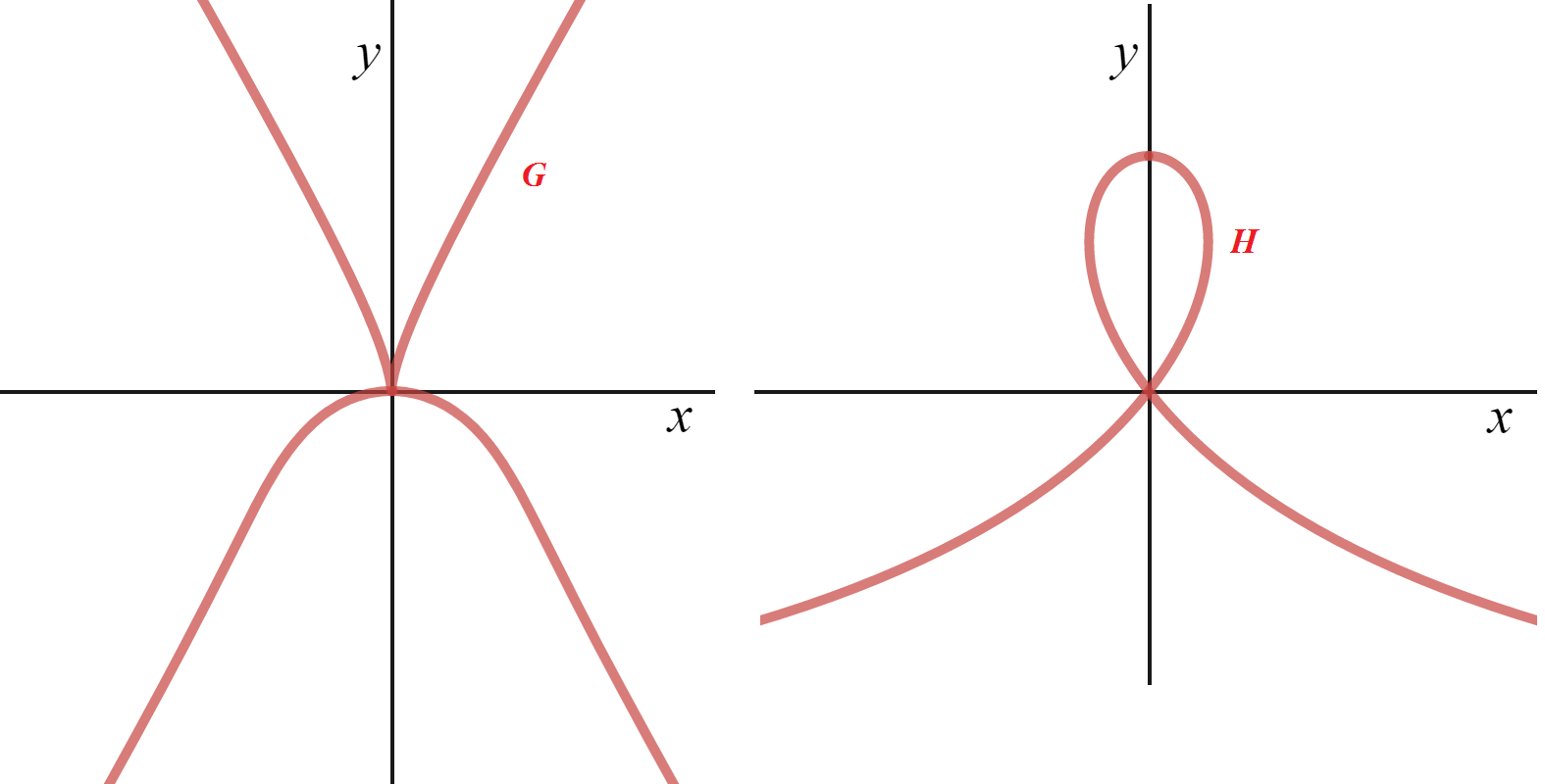
Auxiliary Curves G and H

Recall that F, the four-petal rose, has two branches tangent to the x-axis at O. G has only one, and H has none. Note that we remove a factor of y passing from F′ to G, and from G′ to H.

The full computation of I(E∩F) looks like this:

I(E∩F) = I(E∩F′) = I(E∩yG),  by (7)
I(E∩yG) = I(E∩y) + I(E∩G),  by (6)
I(E∩G) = I(E∩G′) = I(E∩yH),  by (7)
I(E∩yH) = I(E∩y) + I(E∩H),  by (6)
I(E∩H) = m(E) m(H) = 3×2 = 6,  by (5)
I(E∩y) = I(x⁴∩y),  by (7)
I(x⁴∩y) = m(x⁴) m(y) = 4×1,  by (5)
I(E∩F) = I(E∩y) + I(E∩y) + I(E∩H) = 4+4+6 = 14

—the same result we’ve seen before.

I’ll look at Fulton’s other definition in Post 7.

Prev TOC Next