
As I said last time, I’m learning some algebraic geometry, starting with Bézout’s theorem, and using Fulton’s Algebraic Curves and Kendig’s A Guide to Plane Algebraic Curves as the texts. Right now we’re looking at this example from Fulton:


Fig.1
Only 5 intersections (green dots) are visible, but Bézout’s theorem tells us there should be 4×6=24.
Let’s state Bézout’s theorem properly. Suppose E and F are polynomials in two variables over a field k, coprime (equivalently, the curves don’t have a common component—see Fulton §3.6). Then the number of intersections is the product of the degrees, provided:
- k is algebraically closed, and
- We work in the projective plane (thus allowing points at infinity), and
- We count points according to their multiplicity.
As I said last time (and will explain next time), the origin O is an intersection with multiplicity 14. Throw in the other four visible intersections, and we still have 6 missing points.
(By the way: k has become a top choice for the name of ground field, as it’s called. Why k? From the German Körper, body. Why lowercase? Just a guess, but it allows you to use K for an extension field.)
Let’s start with item (1). Fig.1 shows the part of E and F lying in ℝ2. (I’ll use E and F for both the polynomials and the curves. In fact, I’ll be overloading the letters E and F a lot.) What’s happening in ℂ2? Tough to visualize, because E and F are surfaces in a space with four real dimensions, namely ℂ2. But we can take 2d slices of ℂ2, so to speak. Say x=x1+ix2 and y=y1+iy2. Fig.1 displays the real part, i.e., the slice with x2=y2=0. To show (for example) points with x pure imaginary and y real (i.e., x1=y2=0), we can substitute ix for x, getting Fig.2 below. (Up close on the left, and zoomed out on the right.)
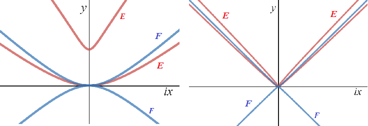


Fig.2
Let’s see what these figures tell us about E; in particular, about E‘s intersections with the horizontal lines y=c. A couple of facts: the top red lobe in Fig.1 extends from y=0 to y=1, and the top red curve in Fig.2 starts at y=1. (Just take my word for it.) For 0<c<1, the real part of E (Fig.1) intersects y=c in two different points. But in ℂ2 there are four intersections. (Bézout! Or the Fundamental Theorem of Algebra.) Now look at Fig.2 on the left: the lower “red smile”, a piece of E, intersects y=c in two points. Our missing two points! In Fig.1, there are no points on E with y>1, but the upper red curve in Fig.2 takes over, providing two more intersections with y=c>1.
For c<0, but not too negative, all four intersections of E with y=c are real, as we see from Fig.1. But when the horizontal line lies below the bottom two lobes of E, we see no intersections in either Fig.1 or Fig.2. That’s because all four values of x are (as it happens) neither real nor pure imaginary.
It’s much the same story for F‘s intersections with horizontal lines. Degree six, so we expect six intersections. Four are real when the line intersects the lobes of Fig.1. Otherwise, all six are imaginary. Two are pure imaginary, always, as you can see from Fig.2. We have a single point with multiplicity 6 at the origin (as we’ll see in the next post).
Now take a look at the right side of Fig.2. It appears that E and F might meet “at infinity”, just the way parallel lines meet at infinity in perspective drawings. That’s our cue to transplant ourselves to the projective plane.
Kendig does a lovely job explaining the projective plane in chapter 2, so I’ll just hit the highlights, and throw in a little art history. (I also recommend Chapter 5 of Stillwell’s The Four Pillars of Geometry.) The technique of perspective appeared in Italy in the 1400s, usually attributed to Brunelleschi (1415), and described first by Alberti in 1435. Take a look at this well-known illustration from Through the Looking Glass:

We have two planes: the chessboard, and the viewing plane (or picture plane). Imagine the viewing plane as a sheet of glass through which you view the chessboard. You paint what you see through the glass on the glass, pixel by pixel. Lacking high-quality sheet glass, Dürer devised a technique using a hinged panel for the viewing plane and a system of threads to record coordinates:

Dürer’s engraving draws our attention to lines passing from the lute through the viewing plane to the artist’s eye. Passing from art to mathematics, we drop the restriction to finite canvases and chessboards. We rename the chessboard plane the object plane. Let O, the origin, be the location of the eye. We extend the line of sight to be infinite in both directions. We now have a 1-1 correspondence between lines through O and points in the viewing plane, except for lines parallel to the viewing plane. This gives rise to a 1-1 correspondence between the object plane and the viewing plane, except for lines parallel to either of the two planes. Lines parallel to the object plane intersect the viewing plane in points that look like infinitely distant points of the object plane.
This diagram portrays the projective correspondence:
The object plane is Z=1, parallel to the XY-plane. The viewing plane is Y=1, parallel to the XZ-plane. The two red dots correspond to each other.
Putting all this together, we have a so-called pencil of lines, all passing through the origin; two planes, so-called affine planes, and a nearly 1-1 correspondence between them, furnished by the pencil. If we extend both planes with lines at infinity, we arrive at a true 1-1 correspondence between two projective planes. OK, but which of our two planes is the projective plane? Why not declare the central participant, the pencil of lines through O, to be “the projective plane”, and the lines to be “projective points”? No reason. So that’s what we do.
Formally speaking, the points of the projective plane over a field k are the lines through the origin in k3. If (X,Y,Z) lies on such a line, then we can parametrize the whole line as (tX,tY,tZ), provided (X,Y,Z) isn’t the origin. Consequently, triple ratios (X:Y:Z) serve as coordinates in the projective plane. These are called homogenous coordinates; traditionally, upper case letters are used for them, with lower case used for affine coordinates.
If we want to make projective points look like points, we intersect the lines with a viewing plane. For example, let’s choose Z=1 as our viewing plane. Any point (X:Y:Z) also has coordinates (X/Z:Y/Z:1), provided Z≠0. So the projective point (X:Y:Z) corresponds to the point (X/Z, Y/Z) in the affine plane Z=1.
The exceptional points, with Z=0, comprise the line at infinity. To see what’s happening there, we change viewing planes, say to Y=1. Now we have a new line at infinity (Y=0), and the old line at infinity has become the x-axis (z=0 in the xz-plane). A point (X:Y:0) has become (X/Y:1:0); that is, (xold/yold, 0) on the x-axis in the xz-plane. A line through O with slope yold/xold in the old viewing plane will pass through this point in the new viewing plane.
OK, what happens to algebraic curves? If E(x,y) is a polynomial, then we homogenize it into a polynomial E(X,Y,Z) by tossing in factors of Z so that all terms have the same degree (and overloading the letter E even more). Taking one of our favorite examples:

The projective completion of E(x,y)=0 consists of all projective points (X:Y:Z) satisfying E(X,Y,Z)=0. To see what it looks like in the Y=1 viewing plane, just dehomogenize by setting Y=1:

If z=0 this becomes 
But now take a look at the right side of Fig.2. It sure looks like parts of E are approaching slopes 1/(±i). Presumably E meets the line at infinity in the two points (±i:1:0).
Let’s homogenize E(ix,y) and then dehomogenize by setting y=1:


If we do the same for F, we get this picture:


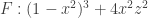
Fig.3
As you can see, E and F have two distinct intersections. As I mentioned last time, these are each triple intersections (not obvious!), so we’ve found all the E-F intersections Bézout promised.
So imaginary points at infinity are not so strange. The real fun starts when we try to make sense of multiplicity. Next time!
