
In 1856 Dirichlet made the following claim in a lecture:
If a bounded surface is given, then one can spread mass continuously over it in one and only one way so that the potential at every point has an arbitrarily prescribed (continuously varying) value…
…This theorem is actually identical with another one from the theory of heat, that one being immediately evident, namely, that if one constantly maintains an arbitrarily prescribed temperature everywhere on the boundary of [a bounded connected region] t, then there is one and only one possible temperature distribution at equilibrium…
…We prove this theorem via a purely mathematical argument. Indeed, it is clear that among all functions u that together with their first derivatives vary continuously in t and assume prescribed values on the boundary of t, one (or more) must exist for which the [an energy] integral … extended over the entire region t attains it smallest value.
Riemann later dubbed this the Dirichlet Principle; he’d already been using it in complex function theory. In 1870, Weierstrass threw a monkey-wrench into the argument. As he said,
on the contrary one can maintain only that the expression in question [the energy integral] has a lower bound, which can be approached as closely as desired, without actually being able to reach it. Accordingly Dirichlet’s mode of reasoning is invalid.
He gave an example of an integral (but not the energy integral) whose possible values, for a suitable class of integrands, had a lower bound but not a minimum.
This episode is famous in the history of mathematics. People found alternate proofs for the results obtained using the principle. In 1899, Hilbert presented a rigorously provable version of the Dirchlet Principle sufficient for the applications. Chapter 9 of Constance Reid’s Hilbert tells the story lucidly, avoiding technicalities. If you want the math full-strength, just look up “direct methods in the calculus of variations”.
A few years back I became curious about the Weierstrass example, and I found the original paper in German. I made a translation into English. That’s my excuse for this post.
In the simplest version, Weierstrass’s example looks like this:

The functions here are

and the integral is
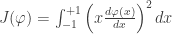
Weierstrass assumes that ϕ and ϕ′ are continuous on the interval and obey the boundary conditions ϕ(–1)=–1, ϕ(1)=1. It’s clear that J(ϕ) cannot be negative. He does an explicit calculation to show that J(fN) can be made arbitrarily small. But this is not hard to see intuitively: for large N, the derivative is close to 0 except for x close to 0, where the factor of x keeps the integrand from getting too big. Approximate fN with the continuous piecewise linear function that is 0 except between –1/N and 1/N, where it has slope N. The integrand for that subinterval of length 2/N is less than [(1/N)·N]2=1, so the integral is less than 2/N.
On the other hand, J(ϕ) cannot be 0. If it were, then ϕ′ would be identically 0, ϕ would be constant, and the boundary conditions would not be satisfied. QED
