
When did logic advance decisively beyond Aristotle? “Boole!” “Frege!” “Peirce!” “Peano!” “Löwenheim and Skolem!” Good arguments can be made for all of these, but to my mind, alternation of quantifiers marked the sea-change. (Now I have to admit I don’t know who first introduced this. Oh well.)
I think of Aristotle’s logic as “always, sometimes, never” logic. The premises and conclusions of his syllogisms can always be cast in the form ∀x P(x) or ∃x P(x), where P(x) is a boolean combination of some sort. The example:
man(Socrates); ∀x(man(x)→mortal(x)); ∴ mortal(Socrates)
Strings of quantifiers ∀∃, ∃∀, ∀∃∀, etc. take this to a new level.
For example, let’s look at uniform convergence. Cauchy flubbed this the first time, when he “proved” that a limit of continuous functions was always continuous. (He eventually got it right. See Jeremy Gray, The Real and the Complex: A History of Analysis in the 19th Century, pp.39ff for the whole story.) The distinction becomes crystal clear with quantifiers:
∀ε>0 ∃N ∀x ∀n>N |fn(x)-f(x)|<ε
versus
∀ε>0 ∀x ∃N ∀n>N |fn(x)-f(x)|<ε
They both say that limn→∞ fn(x) = f(x). But we have ∃N ∀x in one, ∀x ∃N in the other. In the first case, N can chosen independently of x; in the second we must choose x before we know how big to make N.
The ∀∃ sequence occurs every time we say “there are an infinite number of”:
∀n ∃p (p>n ∧ prime(p))
and the ∃∀ sequence anytime we assert the negation, “there are only finitely many”. The two convergence assertions both have the form ∀∃∀. Perhaps you’re thinking, “One is ∀∃∀∀, the other is ∀∀∃∀”. But for many purposes, a block of quantifiers of the same type amounts to much the same thing as a a single one of that type. We’ll see some examples in a moment.
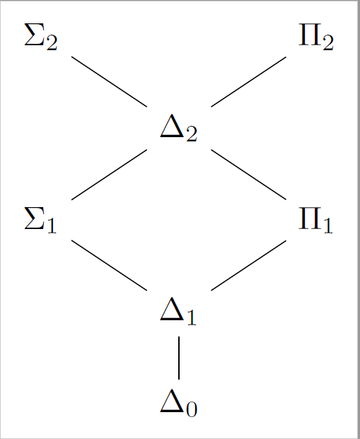
The Borel hierarchy of point-sets implicitly invokes alternating quantifiers. Borel looked at countable unions of closed sets, countable intersections of countable unions of closed sets, etc. Symbolically, ∪, ∩∪, ∪∩∪, etc. (In this case, it’s clear that ∪ and ∪∪ are interchangable, likewise ∩ and ∩∩.) It’s obvious what unions have to do with existential quantifiers and intersections with universal quantifiers. In those days, people mostly used Σ for unions of many things and Π for intersections, following Boole’s use of + and ⋅. So we could write Σ, ΠΣ, ΣΠΣ, etc. Or more briefly, Σn for an alternating sequence of n quantifier blocks starting with a Σ, and Πn for n alternating blocks starting with a Π. To round things out, Δn stands for anything that is both Σn and Πn. Also, it’s convenient to treat Σn and Πn as both contained in Δn+1—imagine a dummy quantifier in front.
Kleene adapted the Borel hierarchy to recursive function theory, calling it the arithmetic hierarchy; from there it made its way into Peano arithmetic. Lévy introduced a similar hierarchy into ZF set theory. Meanwhile, Abraham Robinson and his followers exploited the ∀, ∃∀, ∀∃∀, sequence to the hilt in model theory, where it’s referred to as the ∀n/∃n hierarchy.
I’ve been way too vague about what the Σn/Πn hierarchy classifies. For starters, it classifies formulas. Any formula of first-order logic has a logically equivalent formula in prenex normal form:

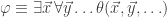
where I’ve written 


For recursion theory, we change the base level. Instead of saying that 
(Incidentally: once again we can ignore the distinction between ∀∀ and ∀, or between ∃∃ and ∃, because we have recursive pairing functions. Suppose 〈x,y〉 is the pair (x,y) coded up as a single number, and coord-1 and coord-2 disassemble coded pairs. Then we can replace ∃x∃y φ(x,y) with ∃z φ(coord-1(z),coord-2(z)) , for example.)
So: the Δ0 (=Σ0=Π0) relations are just the recursive relations, and if you have a modicum of recursion theory (aka computability theory), you should see that the Σ1 relations are the recursively enumerable (r.e.) relations, the Π1 relations are their complements, and the Δ1 relations are also the recursive relations. Simplest example: to see if x belongs to the set defined by ∃yθ(x,y), we just go through the computations for θ(x,0), θ(x,1), θ(x,2),…, and if a y turns up making θ(x,y) true, why then x is in luck! But if x is out of luck, we might never find out—unless there’s another equivalent definition, say ∀yη(x,y). Then we’ll discover x’s bad fortune as soon as a y turns up with η(x,y) false.
So far we’ve just been looking at relations on ℕ. Now let’s cross the bridge to the neighboring borough of Peano Arithmetic. For formulas in the language of PA, we have the ∀n/∃n classification, courtesy of model theory. But people soon realized that we get a more useful hierarchy by letting the base level, Δ0, be all formulas where all quantifiers are bounded. For example, here’s a Δ0 formula δ(n) (of no special significance):
∀q<n ∃k<n ∃r<q (¬q=0 → n=qk+r)
On the one hand, any Δ0 formula clearly defines a recursive predicate. The converse does not hold. But go one level up, and we have two lovely results:
A relation on ℕ is r.e. if and only if it is defined by a Σ1 formula.
A relation on ℕ is recursive if and only if
it is defined by both a Σ1 formula and a Π1 formula.
Proving this takes some serious number theory chops; Gödel showed it using the Chinese Remainder Theorem, in his famous paper on the Incompleteness Theorem.
We still have one foot in ℕ-land. Time to move fully over to PA. A formula φ is Σn(PA) if it is provably equivalent (using PA) to one in Σn form, i.e., an ∃n prefix in front of a Δ0 formula. Likewise for Πn(PA). Finally, it is Δn(PA) if it is both Σn(PA) and Πn(PA). Note: a formula can’t be in both Σn and Πn forms (unless n=0), so it doesn’t make sense to speak of a Δn formula for n>0.
I should also define Σn(N) / Πn(N) / Δn(N), for a model N of PA. A relation on N is Σn(N) if it’s defined by a Σn formula, ditto Πn(N), and Δn(N) as usual means both Σn(N) if and Πn(N). A formula in L(PA) is Σn(N) if it defines a Σn(N) relation on N. In other words, φ is Σn(N) if 
All these words, and we’re just getting to the fun part! To be continued…

Bounded by any closed term made from the parameters, or bounded by any single parameter?
Either way, how powerful are such formulas (in PA)? For example, can they express:
“x to the power y = z”?
“x encodes a satisfiable instance of SAT” (using some encoding a complexity theorist would deem reasonable, i.e. of polynomial size in the usual notion of SAT instance size)?
or the somewhat equivalent
“x encodes a 3-colorable graph”?
or even
“x encodes a correct halting computation of the Turing machine m on the input i, with result r”?
I should add that, as a programmer, it’s obvious to me roughly how to express any of those predicates in PA, provided I can use “high bounds” in the quantifiers, such as (at worst) 2^{poly(x,y,z)} where poly is some polynomial. The part that’s not obvious, without working it out and perhaps using some clever tricks, is just how low those bounds in the quantifiers could go.
(If some of these predicates can only be defined with bounds too high to count as Δ_0, then a “kluge” to make an almost-as-good Δ_0 formula is just to throw in one more parameter p which will be verified as higher than (say) 2^x for each other parameter x, and then the quantifiers can all use p as their bound. But it would be nice if that wasn’t needed!)
BTW, by “closed term” I just meant “term made of parameters, 0, plus, times, and successor”. Maybe I am not using “closed term” correctly.
Here is a way to effectively extend the bounds of ‘∃’ quantifiers in a Δ_0 formula with a parameter n, from n to any poly(n) — just add quantified variables bounded by n (or n – 1) for the base and all the digits of a base-n number, with that number computed inside. That is:
∃ x < n^3 s.t. P(x)
is equivalent to
∃ b <= n, x2 < n, x1 < n, x0 < n s.t. P(x2bb + x1*b + x0)
(I saw a hint of this trick in some paper I looked at recently.)
I didn’t yet work out how to extend it to ∀ (or whether it can be).
(What wordpress formatted as “x2bb” is supposed to be x2 times b times b.)
I’m 95% sure this trick works for arbitrarily nested ∃ and ¬, which means it works for ∀.
I didn’t yet work out whether this means SAT is Δ_0, but I suspect it does (i.e. that poly-sized bounds in the parameters are high enough to express it).