
The Resultant, Episode 2
By now you know the characters: the polynomials E(x) (degree m) and F(x) (degree n) with coefficients in an integral domain R, its fraction field K, and the extension field L of K in which E and F split completely:
E(x) = a(x–u1)···(x–um), F(x) = b(x–v1)···(x–vn)
And we have our resultant resx(E,F), an element of R, which is 0 if and only if E and F have a common root in L. When R=k[y] and K=k(y), that common root would be an algebraic function of y—what we’ve been calling a branch.
We assume, by the way, that m and n are both positive.
(In the Inside-the-Episode example, with the roles of x and y switched, we have the branches 

Even when E and F have no common branch, the resultant still has news to impart, when R=k[y]. We can have ui(y)=vj(y) at particular values of y (for some i and j). So resx(E,F), a polynomial in y, tells us the possible values of y at the intersections of the curves E and F. (Inside-the-Episode example: the intersections occur at x4=0.)
Let’s look at the abstract situation, and see what we can glean from that. Our theme: “As above, so below.” That is, the resultant belongs to R, while the common root (if any) belongs to L. What other assertions about L translate down to R?
First observation: E(x) and F(x) have a common root in L if and only if they have a common factor over L that’s not a constant.
Obviously a common root implies a nonconstant common factor, by the so-called factor theorem: if r is a root of f(x), then (x–r) is a factor. But the converse is also easy: since E(x) factors completely in L, so does a nonconstant common factor, since L[x] is a UFD (because L is a field). So our common factor has a root in L, which naturally must also be a root of F(x).
“Having a common root” doesn’t translate between R and L, or even between K and L. But “having a nonconstant common factor” might. Obviously it translates upwards. How about downwards? In other words, if E(x) and F(x) have no nonconstant common factor in R[x] (or K[x])—if they are coprime there—are they coprime in L[x]?
Remarkably, yes, when R is a UFD. (Remarkable because being irreducible isn’t preserved as we “go upwards”. Standard example: x2+1 is irreducible in ℝ[x] but not in ℂ[x].) From Gauss’s lemma we get: “coprime in R[x]” implies “coprime in K[x]”. Now, K[x] is a PID, so if E and F are coprime, then pE+qF=1 for some polynomials p,q∈K[x]. But that equation still holds in L[x], and it implies that any common factor of E and F divides 1. So it’s a unit, and E and F are coprime in L[x].
The expression pE+qF has made its entrance onto the stage! It will play a major role in the rest of “The Resultant” miniseries, and even beyond.
Observe: if E and F are not coprime, then E=AB and F=BC for some A≠0, C≠0, and nonconstant B. So EC=(AB)C=A(BC)=AF, or EC–AF=0. Therefore there are nonzero polynomials p and q such that
pE+qF=0
with deg(p)<deg(F), deg(q)<deg(E)
Conversely, if we have pE+qF=0 with the degree inequalities, then pE=–qF, so E divides qF. E doesn’t divide q because deg(q)<deg(E). Using unique factorization, it follows that some irreducible (nonconstant) factor of E divides F, so E and F are not coprime. A bonus: this argument works equally well in R[x], K[x], and L[x].
The upshot: being coprime and not being coprime both boil down to the existence of certain polynomials in K[x], and if they exist down in K[x], they also exist up in L[x].
The “pE+qF=1″ argument relied on K[x] being a PID. When R=k[y], the integral domain R[x] (aka k[x,y]) isn’t a PID, just a UFD. But the equation pE+qF=1 in K[x] still tells us something about R[x]. Namely, K is the fraction field of R, so we can clear the denominators in the coefficients of p and q, getting PE+QF=D in R[x], with D in R.
Remember the coordinate ring Γ(E∩F) of post 7? The quotient k[x,y]/(E,F)? Notice that the ideal (E,F) of k[x,y] is the set {PE+QF : P,Q∈k[x,y]}, and its smallest enclosing ideal in K[x] is {pE+qF : p,q∈K}, where K=k(y).
With all this as motivation, we’re ready for the final plot twist of Episode 2. Let’s look at the homomorphism
K[x]⊕K[x] → K[x]
⟨p,q⟩ ↦ pE+qF
Call it Φ. If we regard K[x]⊕K[x] and K[x] as vector spaces over K, then Φ is a linear operator. This turns our thoughts to its null space, its image, stuff like that. K[x] is infinite-dimensional over K. Which is OK, but finite dimensional vector spaces are easier to deal with. But now recall the degree inequalities from above: deg(p)<deg(F)=n, deg(q)<deg(E)=m. Let’s write Km[x] for the space of all polynomials over K of degree <m, likewise Kn[x]; these have dimensions m and n as vector spaces over K. So we can restrict Φ to get
Kn[x]⊕Km[x] → Km+n[x]
⟨p,q⟩ ↦ pE+qF
We observed earlier that E and F are not coprime if and only if pE+qF=0 for some nonzero p∈Kn[x] and q∈Km[x]. Our restricted Φ is singular if and only if E and F are not coprime.
It’s easy enough to write the matrix for the restricted Φ, over the bases {1,…,xn–1; 1,…,xm–1} and {1,…,xm+n–1}. You might think I repeated some elements when I wrote {1,…,xn–1; 1,…,xm–1}. Not so. We get the basis of Kn[x]⊕Km[x] by concatenating the bases of Kn[x] and Km[x]. So (for example) those two 1’s represent different basis elements, namely ⟨1,0⟩ and ⟨0,1⟩, sent by Φ to E and F respectively.
Suppose E(x)=a0+···+amxm, F(x)=b0+···+bnxn. Here’s the matrix, picking the special case m=2 and n=3, with the bases shown above and at right:
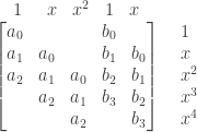
Blank entries are zeros. For example, the basis element ⟨x,0⟩, topping the second column, is sent to a0x+a1x2+a2x3; the basis element ⟨0,x⟩, topping the last column, is sent to b0x+b1x2+b2x3+b3x4.
This is called the Sylvester matrix. (Usually transposed, and often with the rows/columns rearranged. Conventions differ. I’ll switch to the traditional form in the next post.)
The determinant of the Sylvester matrix is therefore zero, when and only when E and F have a common nonconstant factor. Hey, that’s just like the resultant! Maybe the Sylvester determinant equals the resultant?
Indeed it does. (Within a factor of ±1, depending on conventions). We’ll see why in Episode 4.
